
← Back to the 4d application (GUI)
The 4D full-screen browser — inspect a 4D-STEM dataset
The 4D full-screen browser opens whenever you open a 4D-STEM
dataset in 4d's native HDF5 format (an .h5 file,
e.g. from the Library or a results panel). It fills the screen with a split
view: on the left the real-space side — the scan
positions and the reconstructed image — and on the
right the reciprocal-space side — the individual
diffraction pattern recorded at the current scan position.
Simply moving the mouse across the left panel selects the nearest scan
position and updates the right panel live, so you can "fly" over your specimen
and watch the diffraction patterns change.
Across the top runs a control bar with four groups — scan-coordinate loading, Shadow-image calculation (which also holds the BF and DF virtual detectors), iDPC and iCOM calculation, and Circle positioning. The small square ? help button in the top-right corner, just below the Circle positioning panel, opens this manual page.
The window, region by region
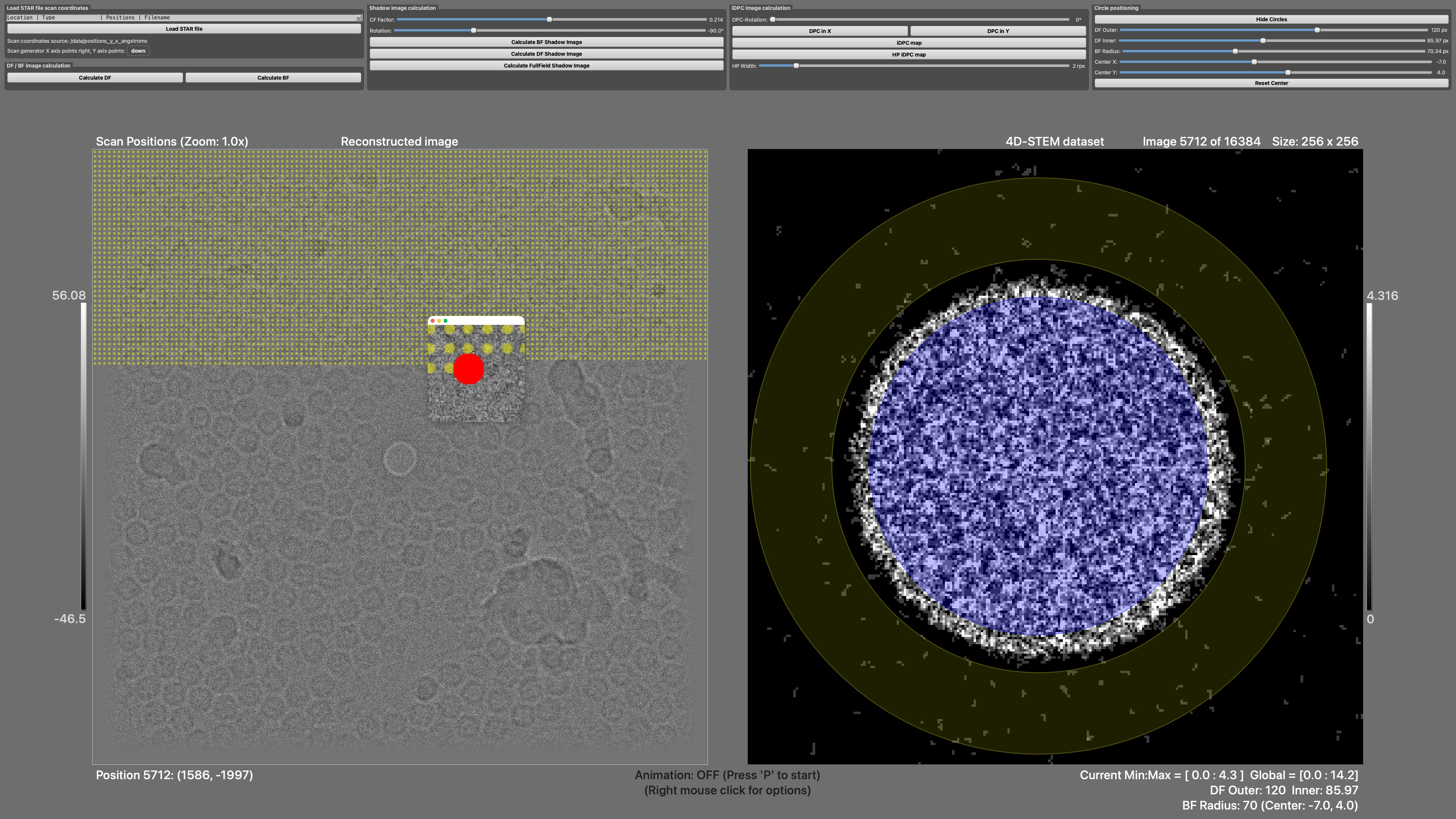
The screenshot below shows the full-screen browser with a cryo-EM 4D-STEM dataset loaded. Each region is marked with a number; the legend that follows explains what each one is and does.
 1
2
3
4
5
6
7
8
9
10
11
18
12
13
14
15
16
17
1
2
3
4
5
6
7
8
9
10
11
18
12
13
14
15
16
17
| # | Region | What it is and does |
|---|---|---|
| 1 | Load STAR file scan coordinates | Pick a scan-position .star file from the project and load it, replacing the coordinates stored in the HDF5 file. |
| 2 | Scan-coordinate source | The file or HDF5 dataset the current scan coordinates come from, and the scan-generator axis convention — X points right, Y points down or up. The button toggles the Y direction; every reconstruction flips with it. |
| 3 | Shadow image calculation | All real-space reconstructions except iDPC/iCOM. The CF Factor and Rotation sliders control the shadow-image reconstruction and show a live preview while dragged. BF_Shadow / DF_Shadow compute the two shadow images, BF / DF the virtual-detector images, and the bottom row the two difference images BF_Shadow − DF and Shadow − Mean, whose subtracted image is weighted by the Subtr. Contrast slider. |
| 4 | iDPC and iCOM image calculation | Differential phase contrast: DPC in X / DPC in Y compute the two half-circle shift maps and COM in X / COM in Y the centre-of-mass equivalents; iDPC map and iCOM integrate them into a phase image, and High-pass map adds a Gaussian high-pass (width set by the HP Width slider). The Rotation slider corrects the scan-vs-detector rotation. See below. |
| 5 | Circle positioning | Show/hide the circle overlays and set the DF Outer, DF Inner and BF Radius in detector pixels, plus the common Center X/Y offset (also movable with the arrow keys). Reset Center returns the center to (0, 0). The ? help button sits directly below this panel. |
| 6 | Scan-position overlay | Every scan position drawn as a yellow dot over the reconstructed image. The Space bar cycles its transparency (invisible → 40% → 80%), S opens its display settings (dot size, probe diameter, animation speed…), and the mouse wheel zooms (1–20×, cursor-centred; the current zoom is shown in the title above). |
| 7 | Reconstructed image | The real-space result panel ("Reconstructed image"). It shows the most recent DF, BF, Shadow or iDPC reconstruction — or the live shadow preview while you drag the CF/Rotation sliders. Hovering here moves the current scan position. |
| 8 | Zoom window | A click into the image opens the floating magnifier window centred on the clicked point; drag to move it around. The solid red dot (visible inside it here) always marks the current scan position. |
| 9 | Grey-value scale & histogram (left) | The displayed grey-value range of the reconstructed image (min at the bottom, max at the top), with the image’s histogram drawn to the left of the bar, perpendicular to the grey axis. Drag along the bar to display only that grey range; double-click it to return to the full range. |
| 10 | Position read-out | The current scan-position index and its (x, y) scan coordinates. |
| 11 | Status hints | Animation status ("Press 'P' to start") and the reminder that a right mouse click opens the options menu. |
| 12 | Diffraction pattern | The 4D-STEM detector frame recorded at the current scan position ("4D-STEM dataset"). Hovering over it shows the detector value under the cursor, taken from the data themselves (while the dataset is held in memory), so neither the Color tool's inversion nor the displayed contrast range affects it. |
| 13 | BF disk overlay | The bright-field disk (blue) defined in the Circle positioning panel — the integration region for BF and BF_Shadow. |
| 14 | DF annulus overlay | The dark-field annulus (dark yellow) between DF Inner and DF Outer — the integration region for DF and DF_Shadow, the DF image subtracted in BF_Shadow − DF, and the DPC deflection maps. COM does not use the annulus: it takes the intensity-weighted centre of the whole disk out to DF Outer, bright-field disk included, so DF Inner plays no part in it. Toggle both overlays with C. |
| 15 | Grey-value scale & histogram (right) | The displayed intensity range of the diffraction pattern, with its histogram to the right of the bar. Drag along it to restrict the display to a grey range, double-click to reset to the full range. The Color tool (O) and B/N (brighter/darker) do the same numerically. |
| 16 | Image index & size | The current pattern number, the total number of patterns, and the detector frame size in pixels. |
| 17 | Value read-outs | The current and global min/max of the pattern intensities, and the present DF Outer/Inner and BF radius/center values. |
| 18 | Value under the cursor | Val: shows the grey value of the reconstructed image under the mouse pointer, in the same units as the scale bar (9). It follows the cursor live and disappears when the pointer leaves the image. |
The Image Statistics window (key A)
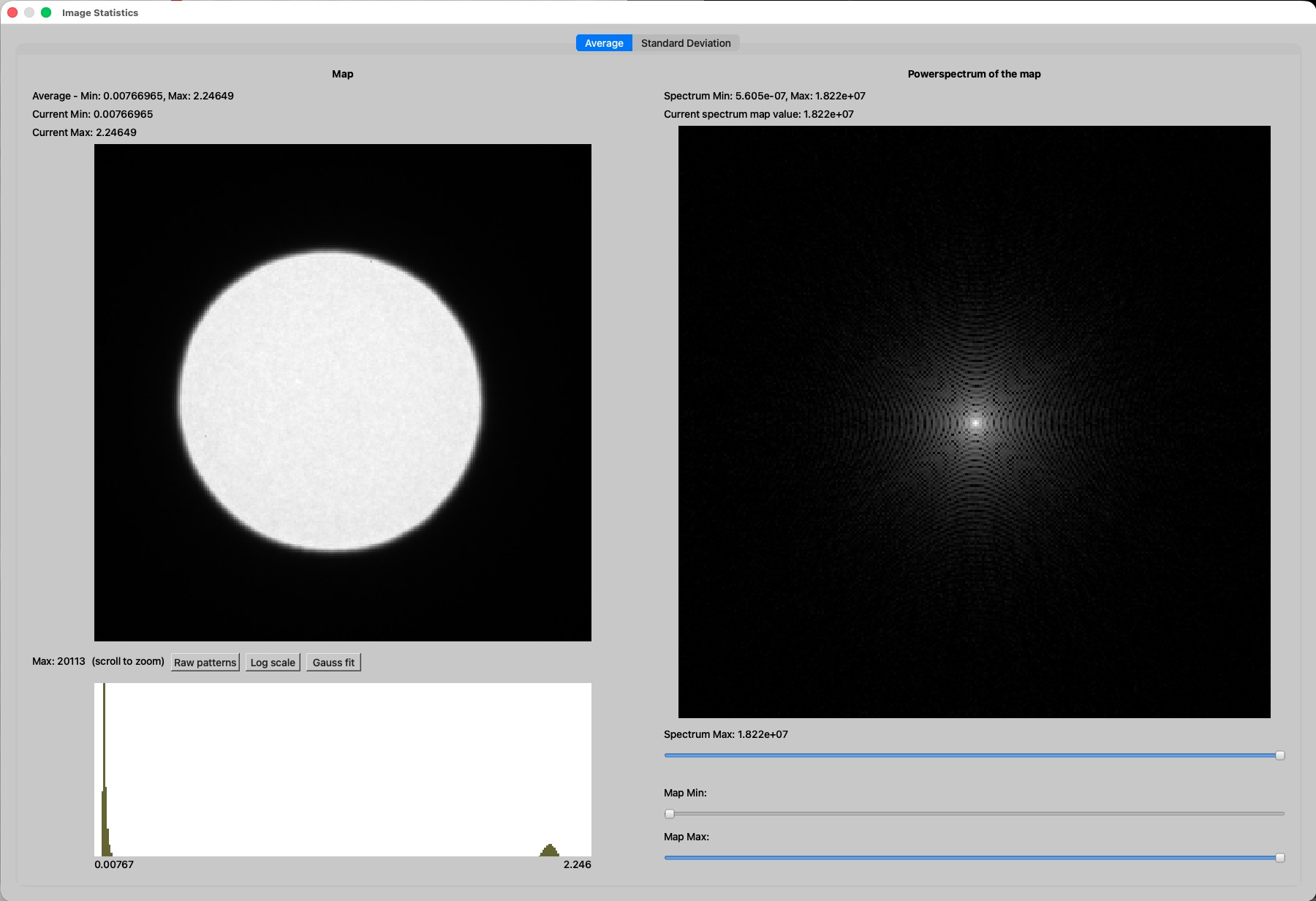
Pressing A opens the Image Statistics window with the average and standard-deviation maps over all diffraction patterns of the dataset — useful for checking the detector illumination, finding the bright-field disk radius, and judging overall data quality.
 1
2
3
4
5
6
7
1
2
3
4
5
6
7
| # | Region | What it is and does |
|---|---|---|
| 1 | Average / Standard Deviation tabs | Switch the map between the per-pixel average over all patterns and the per-pixel standard deviation. |
| 2 | Map | The selected statistics map. With the average map, the bright disk is the direct beam — read its radius here to set BF Radius in the Circle positioning panel. |
| 3 | Histogram controls | Raw patterns switches the histogram to the raw pattern values, Log scale toggles a logarithmic count axis, and Gauss fit fits a Gaussian to the peak. Scroll over the histogram to zoom. |
| 4 | Histogram | The grey-value histogram of the map (or of the raw patterns), with the displayed min/max below. |
| 5 | Power spectrum | The power spectrum of the map — a quick check for periodic artefacts and for the information content of the average pattern. |
| 6 | Spectrum Max slider | Sets the upper display limit of the power spectrum to bring out weak features. |
| 7 | Map Min / Map Max sliders | Set the displayed grey-value range of the map on the left. |
Keyboard shortcuts
| Key | Action |
|---|---|
| mouse move (left panel) | Select the nearest scan position — the diffraction pattern follows the cursor live. |
| L / K | Step to the next / previous pattern in the stack. |
| 0 / 9 | Jump to the first / last pattern. |
| ← ↑ → ↓ | With the circle overlay visible (C): move the circle center in 0.1-pixel steps. With the cursor over the scan plot: step to the nearest scan position in that direction. Otherwise: previous/next pattern. |
| P | Start / stop the animation that plays through the patterns along the scan. |
| + / − | Speed up / slow down the animation. |
| Shift + / Shift − | Increase / decrease the animation step size (skip more / fewer positions per frame). |
| A | Open the Image Statistics window (average / standard-deviation patterns with histogram and power spectrum). |
| D | Toggle the display of average-subtracted patterns (each pattern minus the dataset average — enhances the weak scattered signal). |
| C | Show / hide the BF and DF circle overlays (and the Circle Definition controls). |
| S | Open the scan-position display settings (dot size, transparency, probe diameter, animation, zoom, coordinate convention). |
| Space | Cycle the scan-position overlay transparency: invisible → 40% → 80% → invisible. |
| I | Display coordinate info under the cursor. |
| O | Open the contrast / brightness (color lookup) tool. |
| B / N | Quick-adjust: brighter / darker. |
| . / , | Zoom in / out. |
| M | Show the mouse-button assignment overlay. |
| G | Save a screen shot. |
| H | Toggle the built-in help overlay. |
| Ctrl+F | Toggle full-screen / windowed display. |
| Esc | Close the browser window. |
The right mouse click (and other mouse actions)
A right mouse click anywhere in the browser opens the 4D Viewer options menu (also reachable with Ctrl + left click). It collects all the actions above in one place, with their shortcuts shown:
| Menu entry | Shortcut | What it does |
|---|---|---|
| Show Full Screen | Ctrl+F | Toggle between full-screen and windowed display. |
| Display Coordinate Info | I | Show the coordinate information tool. |
| Zoom › Zoom In / Zoom Out | . / , | Change the display magnification. |
| Adjust Contrast/Brightness | O | Open the color-lookup tool for the displayed grey values. |
| Quick-Adjust Brightness › Brighter / Darker | B / N | One-step brightness changes. |
| Show Mouse Button Assignment | M | Display what each mouse button does. |
| Screen Shot | G | Save an image of the current display. |
| Play Animation | P | Start/stop playing through the diffraction patterns. |
| Navigation › First / Last / Previous / Next Image | 0 / 9 / K / L | Move through the pattern stack. |
| Settings | S | Open the scan-position display settings. |
| Circle Definition | C | Show/hide the BF/DF circle overlays. |
| Cycle Scan Position Transparency | Space | Fade the yellow scan-position dots. |
| Show Average and StdDev Patterns | A | Open the Image Statistics window. |
| Show Baseline-Subtracted Patterns | D | Toggle average-subtracted pattern display. |
| Help | H | Toggle the built-in help overlay. |
| Close | Esc | Close the browser. |
Other mouse actions:
- Left click (over the images) — open the floating zoom window magnifier at the clicked point; keep the button pressed to drag it around.
- Mouse wheel over the left panel — zoom the scan-position plot (1–20×), centred on the cursor; the reconstruction under the dots zooms along.
- Middle drag / Alt + left drag — pan the zoomed scan-position plot; the reconstruction under the dots moves along.
- Hover over the diffraction pattern — read out the pixel value under the cursor.
- Hover over the reconstructed image — read out its grey value as Val: above the top-right corner of the image.
- Drag on a grey-value bar (either side) — display only the picked grey range of that image.
- Double-click a grey-value bar — reset that image to its full grey range.
The reconstructions: DF, BF, Shadow and iDPC
All four reconstructions turn the 4D dataset (a 2D diffraction pattern for every 2D scan position) into a 2D real-space image displayed in the left panel. They differ in which part of each pattern they use and how they turn it into contrast. The BF disk and DF annulus are defined once, in the Circle positioning panel, and shared by all of them.
Circle positioning — defining the detector regions
Toggle the overlays with Show/Hide Circles (key C) and set, in detector pixels: the BF Radius (blue disk — the unscattered "bright-field" beam), and the DF Inner/DF Outer radii (dark-yellow annulus — the scattered "dark-field" signal). Center X/Y shifts both overlays together to compensate a de-centred diffraction pattern; with the overlay visible, the arrow keys nudge the center in 0.1-pixel steps. Use the average map of the Image Statistics window to measure the disk radius and center precisely.
BF and DF images — virtual detectors
The BF and DF buttons — in the second row of the Shadow image calculation panel — emulate the classical STEM detectors: for every scan position, the diffraction pattern is integrated over the BF disk (BF image) or over the DF annulus (DF image), and the integral becomes the grey value of that scan position in the reconstructed image. Bright-field contrast is dominated by absorption/phase effects of the transmitted beam; dark-field contrast highlights strongly scattering (e.g. heavier or thicker) regions. The calculation runs progressively — the image sharpens as more positions are evaluated, and the grey-value scale bar next to the image (9) follows it, always showing the range currently displayed.
Both maps hold one value per scan position. What is drawn is a resampled copy of them: the map is generated with between 256 and 4096 pixels per axis, so a small scan is upscaled to blocks of identical pixels and a scan larger than 4096 positions along an axis is downsampled. The scan-position dots mark the centres of the blocks. The maps are displayed over a range of mean ± 2 σ of the integrated intensities, stretched by the Contrast and Brightness settings of the scan-position dialog (S).
Shadow images — magnified projection from overlapping disks
The shadow (or "shadowgraph") reconstruction exploits the fact that with a defocused or convergent probe, each bright-field disk is a small shadow image of the specimen area around the probe position. The algorithm places every pattern's selected region — mean-subtracted — at its scan position on a large canvas and sums the overlaps:
- CF Factor — the conversion factor from scan coordinates to canvas pixels. It sets the magnification of the shadow image: a larger CF spreads the scan positions further apart, producing a larger, more magnified image. The canvas spans the scan extent times CF plus a border of one diffraction pattern; anything beyond 8192 pixels per axis is centre-cropped to bound memory use.
- Rotation — rotates each pattern about its center to compensate the rotation between scan axes and detector axes. When the rotation (and CF) are correct, features from overlapping disks reinforce instead of blurring.
- Live preview — while you drag either slider, a small white-framed window in the image center shows the reconstruction live. Its size adapts so one preview frame is computed per second; when you pause the slider, increasingly larger frames are computed until the whole image is covered, and when you release the slider the full image is calculated.
- BF_Shadow — the reconstruction from the bright-field disks: each pattern is masked to the BF disk, its mean inside the disk is subtracted, and the result is placed at the scan position.
- DF_Shadow — the same from the dark-field annulus between DF Inner and DF Outer, giving the scattered-signal shadow image.
- Shadow − Mean — uses the entire pattern with no masking, subtracting the dataset-average pattern from every individual pattern before placing it. What survives is the position-dependent part of the signal. Neither a BF nor a DF shadow image is computed here, so the subtracted image is the mean pattern, not a dark-field reconstruction.
- BF_Shadow − DF — the BF shadow image with the DF image subtracted, to remove mass-thickness contrast from the shadow reconstruction. The DF image is computed separately on the scan grid and then registered onto the shadow geometry: the output is cropped to the scan-position area so both images cover the same field of view, patterns are placed with their BF disk centre (not the pattern centre) on the scan position, and the summed disks are divided by their coverage so the amplitude is the same in the middle and along the edges. Both images are rescaled to a common range before the subtraction.
- Subtr. Contrast — weights the subtracted (second) image in both difference modes, from 0.1 to 10 with a default of 0.5. At 1.0 the full second image is subtracted. Releasing the slider recomputes whichever of the two differences was calculated last.
iDPC and iCOM — integrated differential phase contrast
Differential phase contrast measures the deflection of the beam by the local electric field of the specimen. For every scan position, the annular region of the pattern is split into two half-circles and their mean intensities subtracted:
- DPC in X — left-half minus right-half → horizontal deflection map.
- DPC in Y — top-half minus bottom-half → vertical deflection map.
- COM in X / COM in Y — the same two components measured as the intensity-weighted centre of mass of the pattern instead of a half-circle difference. The COM shift is the more quantitative estimator of the beam deflection; the half-circle difference is faster and more robust against a few hot pixels.
- Rotation — rotates the half-circle split line and the COM projection axes to compensate the scan-vs-detector rotation; adjust it until edges in the DPC maps look symmetric rather than sheared.
- iDPC map — treats (DPCx, DPCy) as a gradient field and integrates it in Fourier space (F(k) = i(kxFx + kyFy) / k²). For a thin specimen the result is proportional to the projected electrostatic potential — a directly interpretable phase image with high dose efficiency.
- iCOM — the same integration applied to the COM maps.
- High-pass map — the integrated map followed by a Gaussian high-pass filter (1 − e−k²/2σ², with σ = HP Width in reciprocal pixels) that removes the slowly varying background the 1/k² integration amplifies.
The grey-value bars — histogram and display range
Each of the two images carries a vertical grey-value bar: white at the top for the maximum, black at the bottom for the minimum, with the two values written above and below it. The histogram of the displayed image is drawn alongside the bar, perpendicular to the grey axis and pointing away from its image — to the left of the bar for the reconstructed image, to the right of the bar for the diffraction pattern. Counts are square-root scaled so that a single dominant peak does not flatten the rest of the distribution.
- Drag along a bar (on the bar itself or over its histogram) to pick a grey range. The picked band is shown while you drag, with everything outside it dimmed; on release, only that range is displayed and the labels, the histogram and the Val: read-out switch to the new range. Dragging again narrows the range further.
- Double-click a bar to return to the full grey range of that image.
On the diffraction-pattern side this is the same display range that the Color tool (O) sets numerically, so the two stay in step; a reset there returns to the full recorded range of the dataset. On the reconstruction side the window is dropped automatically as soon as a new image is calculated, since the new image brings its own grey range.