Ptychoscopy — plan a ptychography experiment
Ptychoscopy is an interactive planning tool for electron ptychography, opened from the Planning tab (4D-STEM project mode). Successful ptychographic reconstruction depends on many interdependent choices — probe convergence angle, defocus, camera length, detector binning, scan step, dose — and the right choices differ between the two reconstruction families (direct SSB and iterative ITR). Rather than discovering this by trial and error on the microscope, Ptychoscopy lets you enter your intended settings and immediately see their consequences: the achievable phase contrast-transfer function, the detector geometry and bright-field disk, the beam-overlap map, the dose, and — for iterative reconstruction — a camera-length guide table and a set of pass/fail quality checks. It is based on the method of Skoupy et al. (see Algorithm & theory).
The window, region by region
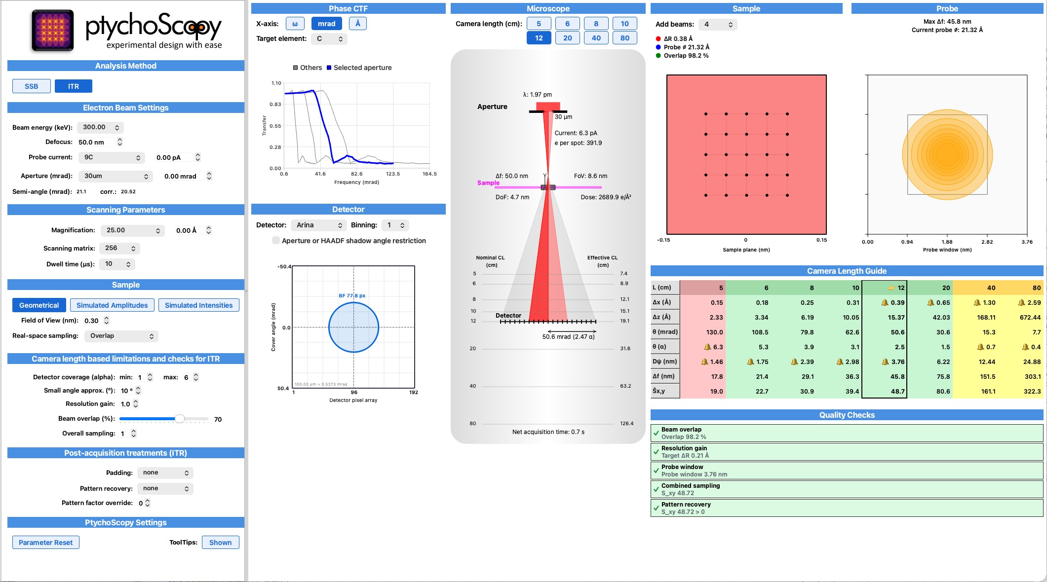
The Ptychoscopy window is a split view: a scrollable parameter panel on the left, and a live visualization panel on the right. The screenshot below (an iterative / ITR example) has each region marked with a number; the legend that follows explains what each one is and does.
 1
2
3
4
5
6
7
8
9
10
11
12
13
14
15
1
2
3
4
5
6
7
8
9
10
11
12
13
14
15
| # | Region | What it is and does |
|---|---|---|
| 1 | Logo | The PtychoScopy logo. Clicking it opens the publication; the small ? on its top-right corner opens this manual page. |
| 2 | Analysis Method | SSB (single-sideband, direct) vs ITR (iterative). This choice reshapes the whole right-hand panel and which checks apply. (ITR is selected in the screenshot.) |
| 3 | Electron Beam Settings | Beam energy (keV), defocus (nm), probe current, and aperture — with a live read-out of the probe convergence semi-angle α (raw and aberration-corrected). |
| 4 | Scanning Parameters | Magnification (which sets the real-space scan step ΔR), the scanning matrix (N×N number of positions), and the dwell time per position. |
| 5 | Sample | How beam overlap is modelled — Geometrical (with a field-of-view and step/overlap/oversampling read-out) or Simulated amplitudes/intensities (illumination-uniformity map). |
| 6 | Limitations & checks (ITR) | The tolerances the iterative quality checks use: detector coverage (min/max α), small-angle limit, resolution gain, target beam overlap %, and overall sampling. |
| 7 | Post-acquisition (ITR) | Zero-padding and pattern-recovery (artificial reciprocal-space upsampling) factors applied before iterative reconstruction. |
| 8 | PtychoScopy Settings | Parameter Reset (restore defaults) and a global tooltips on/off toggle. |
| 9 | Phase CTF | The phase contrast-transfer function vs spatial frequency for the current settings. Switch the x-axis (multiples of α / mrad / Å) and pick the target element whose curve is drawn. |
| 10 | Detector | A diffraction-plane diagram: the bright-field disk over the detector pixel grid, with the angular cover range and pixel size. Choose the detector, its binning, and an optional aperture/HAADF shadow restriction. |
| 11 | Microscope | A schematic ray diagram annotated with wavelength, aperture/semi-angle, defocus, probe current, electrons-per-spot, field of view, dose, depth of focus, the nominal/effective camera-length ladder, and acquisition time. The camera-length buttons above it select the camera length. |
| 12 | Sample map | The beam-overlap map — the scan-position grid with overlapping probe circles — plus a legend for the step size ΔR, probe diameter, and overlap %. Add beams controls how many are drawn. |
| 13 | Probe (ITR) | The probe-window plot with the maximum usable defocus and the current probe diameter — showing whether the probe fits inside the computational window. |
| 14 | Camera-Length Guide (ITR) | A table with one column per camera length and rows for the reconstructed pixel Δx, slice thickness Δz, max detected angle θ (in mrad and α), probe window Dψ, max defocus Δf, and combined oversampling Ŝx,y. Cells turn green/yellow/red to flag values that violate the limits in region 6. |
| 15 | Quality Checks (ITR) | Pass/fail cards (green ✓ / red ✗): beam overlap, resolution gain, probe window, combined sampling, and pattern recovery. Aim for all green. |
images/screenshot-ptychoscopy.png). In SSB mode, regions
13–15 are replaced by a single Camera Length chart (angular cover vs
camera length), and regions 6–7 do not apply.
Step-by-step
- Open Ptychoscopy. In the Planning tab pick the Ptychoscopy tool.
- Pick the reconstruction method (2): SSB for fast direct reconstruction of a limited frequency band, or ITR for iterative reconstruction with super-resolution and depth sectioning.
- Set the beam (3): beam energy, aperture (which fixes the convergence semi-angle α), defocus, and probe current. Watch the semi-angle read-out — α controls both resolution and the CTF shape.
- Set the scan (4): magnification (→ scan step ΔR), scanning matrix, and dwell time. The dose and field of view update in the Microscope sketch (11).
- Set the detector and camera length (10, 11): choose the detector and binning, then a camera length. The detector diagram shows whether the bright-field disk is well sampled.
- Read the CTF (9): choose a target element and x-axis units, and check that the contrast-transfer function reaches the spatial frequency (resolution) you need.
- Check the overlap (5, 12): with Geometrical or Simulated mode, confirm the probe circles overlap enough (SSB needs Nyquist sampling of 2α; ITR needs sufficient signal/uniformity).
- Pass the checks (ITR) (6, 13–15): adjust camera length, binning and step until the Quality Checks are all green and the Camera-Length Guide shows an acceptable reconstructed pixel, probe window, and combined oversampling (Ŝ ≥ 1).
- Use the recommendations. Transfer the chosen semi-angle, defocus, camera length, binning, scan step and dose to your acquisition (and to the Scan Pattern Generator).
Algorithm & theory
Ptychoscopy implements the model of Skoupy, Müller, Pennycook, Guizar-Sicairos, Fabbri, Poghosyan et al., "Ptychoscopy: a user friendly experimental design tool for ptychography", Scientific Reports 15, 24959 (2025). It predicts the achievable resolution, sampling, probe geometry and dose for a set of microscope settings, for the two reconstruction families it models. The relations below (small-angle approximations) are what the tool evaluates; λ is the electron wavelength and α the probe convergence semi-angle.
The two contrast-transfer models
- SSB (single-sideband, direct). The phase CTF is derived
analytically from the overlap of the direct and diffracted probe disks in
reciprocal space. It peaks near
0.9 αand falls to zero at both0and2α— so SSB transfers a limited band and its maximum transferable frequency is at2α. - ITR (iterative). The CTF is not analytic; it is taken from
single-atom simulations (C, Cu or Au). It stays roughly flat from zero up to
about
2αand has an extended tail that enables super-resolution beyond2α, at the cost of iterative computation and higher sensitivity to sampling and dose.
Key relations
| Quantity | Relation | Meaning |
|---|---|---|
| Lateral resolution (SSB) | r = λ / sin(2α) | Finest spacing SSB transfers, set by the 2α band edge. |
| Real-space sampling (SSB) | ΔRSSB = λ / (4α) | Scan step that Nyquist-samples the 2α frequency (avoids aliasing). |
| Reconstruction pixel (ITR) | PixITR = λ / θ ≈ λL / (M·p) | Pixel of the iterative reconstruction, set by the max detected angle θ (camera length L, detector half-width M pixels of size p). |
| Probe-window size | dprobe,max = λ / (2Δθ) ≈ λL / (2·peff) | The probe must fit within half the computational window; peff is the effective (binned) detector pitch. |
| Combined sampling | Δθ · ΔR ≤ λ / 2 ⇔ Ŝ = λL / (2·ΔR·peff) ≥ 1 | Reciprocal- and real-space sampling are coupled; relaxing one demands tightening the other. The check warns when Ŝ < 1. |
| Maximum defocus | Δfmax = dprobe,max / (2α) | Defocus enlarges the probe (fewer positions, less dose) but too much causes reciprocal-space undersampling/aliasing. |
| Depth resolution (multislice) | rz = λ / (2·sin²(θ/2)) | Minimum useful slice thickness for 3D/multislice reconstruction. |
Beam-overlap metrics
For probe diameter dprobe and scan step ΔR, the tool reports three complementary overlap measures:
| Measure | Formula |
|---|---|
| Geometric overlap (%) | (dprobe − ΔR) / dprobe × 100 |
| Linear oversampling | dprobe / ΔR |
| Areal oversampling | π·(dprobe/2)² / ΔR² |
What the tool computes and warns about
- From the microscope calibration (energies, apertures, camera lengths, detector) it derives λ, the semi-angle α (raw and corrected), the probe current and diameter, dose, field of view and depth of focus.
- It draws the method-specific phase CTF so you can match α to the spatial frequency your sample needs.
- It maps the beam positions and probe circles to show real-space sampling / overlap, using either geometry or a simulated probe profile (uniformity).
- It evaluates the camera-length-dependent quantities above and flags violations: reciprocal-space undersampling (Ŝ < 1), a probe larger than half the window, a reconstructed pixel coarser than the step / resolution-gain, a detector angle beyond the small-angle limit, and α outside the requested coverage range.
For the full derivations, validation table, and worked examples, see the open-access publication: Scientific Reports 15, 24959 (2025) (DOI 10.1038/s41598-025-09871-6).