4d — Fibrils

← Back to “Processing sections & scripts”

Fibrils — amyloid fibril detection & analysis

Detect, pick, and analyse amyloid fibrils in cryo-EM micrographs, and maintain their coordinate STAR files. These scripts belong to the Fibril picking project mode, which is designed to sit inside an existing RELION project (pointing at its MotionCorr/ folder): 4d works in a fibrilpicker/ subfolder and never touches RELION's own files.

#	Title	What it does
20	Drift-correct EER file	Calls MotionCor2 to drift-correct an EER movie into a summed micrograph, recording the measured drift.
40	Fibril Picker	Finds amyloid fibrils automatically: a real-space tubeness/Hessian filter proposes candidates, and a Fourier check on the characteristic 4.7–4.9 Å cross-β reflection accepts or rejects them.
50	Fibril Analysis	Reads the picked fibril coordinates, measures each category's average cross-section, fits a Gaussian, and reports width (FWHM), mass-per-length, and fibril lengths.
60	STAR file maintenance	Merges, copies, swaps or deletes the five per-category fibril STAR files.

Pipeline & data flow. The section runs top to bottom and accumulates its results in the dataset folder: 20 turns an EER movie into a drift-corrected micrograph → 40 detects fibrils and writes fibrils.star (category 1) plus the heatmap and dot-map overlays → 50 measures the fibrils in fibrils.star…fibrils5.star → 60 reorganizes those five STAR files. Categories 2–5 are normally filled by hand in the maximized image inspection view, which also displays script 40's heatmap and dot-map overlays. Each script's ? help button opens its entry below.

Pixel size matters. The Fourier test looks for a reflection at a specific resolution, so an accurate pixel size is essential. It is read from the MRC header; when that value is wrong or missing, set particles_pixelsize (Å/pixel) explicitly — the same value the inspection view uses for its FFT resolution rings.

20 — Drift-correct EER file

Purpose

The entry point when you start from raw movies rather than from aligned micrographs. It calls MotionCor2 on the dataset's .eer movie to correct beam-induced motion and produce a summed, drift-corrected image for the picking steps. Its drift statistics also give a first quality criterion for discarding bad micrographs before any picking is attempted.

Parameters

Parameter	Role
`sample_pixel`	Pixel size (Å) of the movie frames.
`KV`	Accelerating voltage (kV), used for dose weighting.
`total_dose` / `frame_dose`	Total exposure and per-frame dose (e/Å²) for dose-weighted averaging.
`movie_stackname`	Name of the movie stack to process.
`MotionCor2_param1…4`	Four free-text argument slots passed straight through to MotionCor2 (e.g. patch layout, grouping, GPU selection) — anything the program accepts can be set here.

Algorithm

Locates the MotionCor2 executable configured for the project and verifies it exists.
Runs it on the EER movie with the pixel size, voltage and dose settings, appending the four free parameter slots verbatim.
Writes the alignment (shift) file and parses it for the drift metrics reported back to the Library table.

Results

Images/files: the drift-corrected micrograph, motioncor2_shifts.aln (alignment file) and LOGS/motioncor2.out (program output).

Values written: drift, drift_longest, drift_deceleration, drift_jitter — sortable in the Library table, so poorly aligned micrographs can be flagged out early.

40 — Fibril Picker

Purpose

The core detection step. It finds amyloid fibrils in a micrograph in two stages: a real-space filter chain that enhances elongated, tube-like features and proposes candidate filament segments, followed by a Fourier test on each candidate that keeps only those showing the characteristic amyloid cross-β reflection at 4.7–4.9 Å. The surviving segments are written as fibril vectors to fibrils.star (category 1), and the intermediate maps become overlays you can inspect.

The result panels

Running the script produces a set of diagnostic images — the whole detection chain, step by step. This is the fastest way to see why a micrograph gave the fibril count it did:

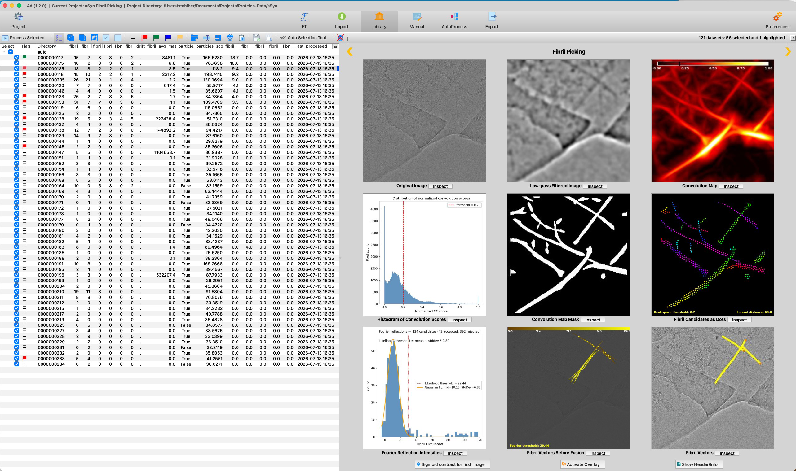Screenshot images/screenshot-fibril-panel.png not found — place it in the manual’s images/ directory.

1 2 3 4 5 6 7 8 9

#	Panel	What it shows
1	Original Image	The input micrograph as read from disk (MRC).
2	Low-pass Filtered Image	The image after binning and smoothing — the basis for the tube detection, with high-frequency noise removed.
3	Convolution Map	The tubeness / Hessian score at every pixel: how strongly each location looks like an elongated ridge. Bright = filament-like. Saved as the heatmap overlay.
4	Histogram of Convolution Scores	The distribution of those scores, with the `particles_threshold_real` cut marked (dashed line) — the key diagnostic for tuning the real-space threshold.
5	Convolution Map Mask	The binary mask after thresholding and cleaning: the pixels accepted as filament.
6	Fibril Candidates as Dots	The mask reduced to traced candidate points, one colour per candidate filament, annotated with the real-space threshold and lateral distance used. Saved as the dots overlay.
7	Fourier Reflection Intensities	The likelihood histogram of the 4.7–4.9 Å reflection over all candidates, with the Gaussian fit and the acceptance threshold. The title reports how many candidates were accepted vs rejected.
8	Fibril Vectors Before Fusion	The accepted candidates as individual straight segments, before collinear pieces of the same filament are merged.
9	Fibril Vectors	The final result: fused fibril vectors overlaid on the micrograph — exactly what is written to `fibrils.star`.

Parameters

Parameter	Role
`particles_pixelsize`	Pixel size in Å/pixel. Overrides the MRC header value; must be right for the Fourier test to look at the correct resolution.
`particles_fibril_width`	Expected fibril width (Å, default 40) — sets the scale of the tubeness filter.
`particles_threshold_real`	Real-space acceptance threshold on the normalized convolution score (default 3.0). Lower = more candidates. Judge it on panel 4.
`particles_fourier_resolution_lower` / `_upper`	The resolution band searched for the cross-β reflection, in Å (defaults 4.7 and 4.9).
`particles_fourier_resolution_back`	Reference/background resolution (Å, default 20) the reflection strength is measured against.
`particles_threshold_fourier`	Acceptance threshold on the Fourier likelihood (default 10).
`particles_threshold_fourier_mode`	`static` uses that fixed threshold; the adaptive mode derives it per image from the fitted likelihood distribution (mean + n·stddev, as annotated in panel 7).
`particles_lateral_exclusion`	Minimum lateral distance (pixels) between accepted filaments — prevents one thick fibril being picked several times side by side.
`particles_angle_tolerance`	Angular tolerance (degrees, default 30) for treating two segments as belonging to the same filament.
`particles_tangential_tolerance`	Perpendicular offset tolerance (pixels, default 1) for the same test.
`particles_fusion_distance`	Maximum end-to-end gap for fusing two collinear segments into one fibril (panel 8 → 9).
`particles_scores_max`	Upper limit on the number of candidate scores carried forward — caps the run time on very crowded images.
`image_min_value`	Minimum grey value used when normalizing the input image.

Algorithm

Preprocess. Bin the micrograph, then apply a Gaussian smoothing, a Kuwahara edge-preserving filter and a bottom-hat transform to flatten the background while keeping thin features.
Enhance tubes. Compute a tubeness (Hessian-based) response at the scale set by particles_fibril_width, giving the convolution map — the filament-likelihood heatmap (panel 3) — followed by a high-pass correction.
Threshold & clean. Cut the score map at particles_threshold_real (panel 4), then clean the resulting binary mask morphologically (panel 5).
Trace candidates. Reduce the mask to filament traces and fit straight lines to them, applying particles_lateral_exclusion so parallel duplicates are suppressed (panel 6).
Fourier test. For each candidate, cut a window along the filament, compute its power spectrum, and measure the intensity in the lower…upper resolution band against the _back background. Candidates below the (static or adaptive) threshold are rejected (panel 7).
Fuse. Merge collinear accepted segments — within particles_angle_tolerance, particles_tangential_tolerance and particles_fusion_distance — into single fibril vectors (panels 8 → 9), and write them out.

Results

STAR file: fibrils.star — the detected fibril segments as category 1, in RELION format (_rlnCoordinateX/Y, _rlnAnglePsi, _rlnAutopickFigureOfMerit). Categories 2–5 are left for manual picking.

Overlays used by the inspection view: fibrilpicker_heatmap.jpg (the Heatmap button) and fibrilpicker_fibril_dot_map.jpg (the Dots button) — see Maximized image inspection.

Diagnostics: the panels above, plus per-window Fourier images (fibrilpicker_fourier_win*_ps.jpg, masked and peak-labelled variants) and the intermediate filter stages (fibrilpicker_debug_00_bin … _07_binary_cleaned).

Values written: fibril_number (total over all five categories), fibril_number1 and particles_fibril_detected — all sortable in the Library table.

50 — Fibril Analysis

Purpose

Turns fibril coordinates into fibril measurements. It reads the picked start/end points from all five STAR files, extracts the image density along each fibril, averages it into a cross-sectional profile per category, and fits a Gaussian to that profile. From the fit it reports the fibril width (FWHM) and the profile integral as a mass-per-length estimate, together with maximum and average fibril lengths. Because each of the five categories is measured separately, they can be used as morphology classes — polymorph 1 in Fibril1, polymorph 2 in Fibril2, and so on — and compared quantitatively.

Parameters

Parameter	Role
`particles_pixelsize`	Pixel size (Å/pixel) — converts the fitted widths and lengths into physical units.
`particles_fibril_width`	Expected fibril width (Å, default 40); sets the width of the extracted cross-section window.
`image_min_value`	Minimum grey value used when normalizing the image before profile extraction.
inputs	`fibrils.star` … `fibrils5.star` in the dataset directory — whatever scripts 40/60 and your manual picking produced.

Algorithm

Reads the fibril start/end coordinates from each of the five STAR files (missing or empty files simply give zero counts).
High-pass filters the binned micrograph against a heavily blurred background copy, so the profile integral measures fibril density rather than the local background level.
For every fibril, samples the image perpendicular to its axis along its whole length and averages those samples into one cross-sectional profile per category.
Fits a Gaussian to the averaged profile; the width follows as FWHM = 2·√(2·ln 2)·σ (implausible fits, below 0 or above 3000 Å, are discarded as 0), and the profile integral becomes the mass-per-length.
Converts the results to nm and nm-based mass-per-length, and measures the fibril lengths from the coordinate pairs.

Results

Images: per category, an overlay of the fibrils on the binned map and the averaged cross-section profile with its Gaussian fit (annotated with the FWHM), plus the high-pass and background images used.

Values written: per category fibril_number1…5, fibril_width1…5 and fibril_mass_per_length1…5; and overall fibril_avg_mass_per_length, fibril_max_length, fibril_avg_length. All appear as sortable Library columns, so you can compare polymorph populations across a whole session.

60 — STAR file maintenance

Purpose

A bookkeeping utility for the five per-category fibril STAR files. Manual picking naturally leaves picks in the "wrong" category — you sort by morphology as you go, change your mind, or want everything collected into one class before export. Rather than editing STAR files by hand, this script performs one of a fixed set of merge/copy/swap/delete operations, and it can be applied to many datasets at once from the Library.

Parameters

Parameter	Role
`fibrils_merge`	The operation to perform (see the table below). `0` means do nothing — the safe default.

Value	Operation
0	Nothing — leave all STAR files untouched.
1	Merge categories 2+3+4+5 into category 2.
2	Merge categories 2+3+4+5 into category 5.
3	Merge all categories 1+2+3+4+5 into category 5.
4	Copy category 1 to category 5 (deletes the old 5).
5	Swap category 1 with category 5.
6	Delete category 5.

Operations 3, 4 and 6 discard data: 4 overwrites fibrils5.star and 6 deletes it. A common use of 5 (swap) is to park the automatic picks of script 40 in category 5 so category 1 is free for manual picking — keeping automatic and manual results side by side for comparison.

Algorithm

Reads whichever of fibrils.star…fibrils5.star exist in the dataset directory.
Applies the selected operation, concatenating the coordinate rows for merges.
Rewrites the affected files with a standard RELION 5 STAR header (_rlnCoordinateX, _rlnCoordinateY, _rlnParticleSelectionType, _rlnAnglePsi, _rlnAutopickFigureOfMerit) and recounts the entries.

Results

Files: the rewritten fibrils.star … fibrils5.star.

Values written: fibrils_number1…5 — the per-category counts after the operation, immediately visible in the Library table and on the inspection view's Fibril1–5 buttons.

Checking the results interactively

The scripts and the interactive maximized image inspection view are two halves of the same workflow. Script 40's heatmap and dot-map are written as image files that the view can overlay on the micrograph with the Heatmap (H) and Dots (D) buttons — so automatic detection and manual picks are directly comparable on the same image:

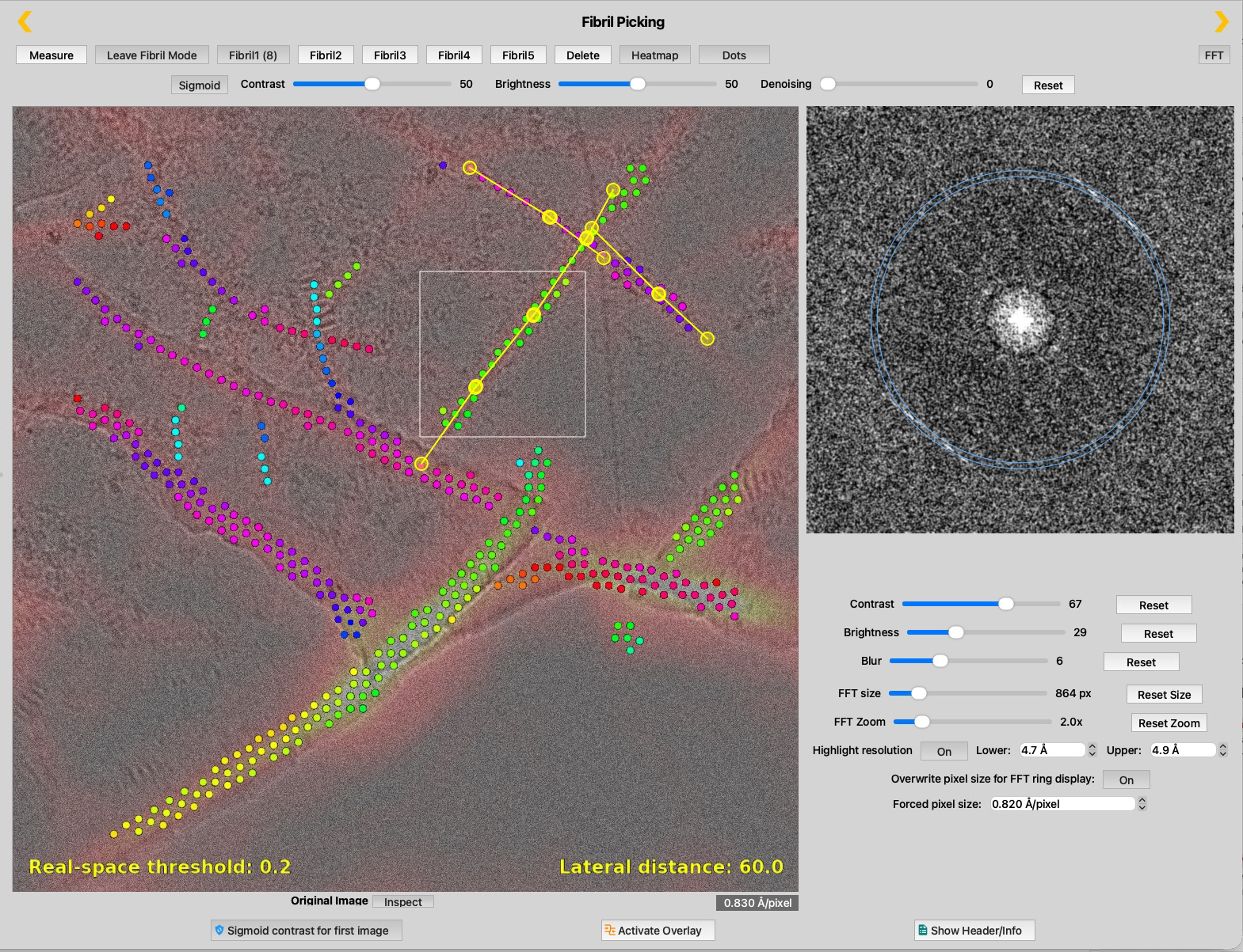Heatmap and dot overlays with manual picks in the inspection view

Screenshot images/screenshot-fibril-heatmap.png not found — place it in the manual’s images/ directory.

1 2 3 4 5

#	Region	What it shows
1	Detected filaments (dots)	Script 40's `fibrilpicker_fibril_dot_map.jpg` — the traced candidate points, one colour per detected filament, over the reddish heatmap of the convolution map.
2	Manual picks	Fibrils picked by hand (yellow lines with circular end markers) drawn on top of the overlays — the direct check of whether automatic detection agrees with your judgement.
3	Real-space threshold	The `particles_threshold_real` value the displayed maps were computed with.
4	Lateral distance	The `particles_lateral_exclusion` value used, in pixels.
5	Live FFT with resolution rings	The Fourier transform of the region under the cursor, with rings at the 4.7–4.9 Å band — the same criterion script 40 applies automatically, here for your own visual check before picking.

A typical fibril workflow

Set up the project in Fibril picking mode, pointing at the RELION project's MotionCorr/ folder.
Drift-correct (script 20) if you start from EER movies; skip it if your micrographs are already aligned. Sort by drift in the Library and flag out the worst.
Check the pixel size. Set particles_pixelsize if the MRC header value is not reliable — everything downstream depends on it.
Tune the picker on one micrograph (script 40): run it, then look at the histogram panels (4 and 7) and adjust particles_threshold_real and particles_threshold_fourier until the accepted/rejected split matches what you see in the final vector panel (9).
Run the picker on the whole session from the Library (or via AutoProcess) with those settings.
Inspect and correct. In the maximized inspection view, switch on Heatmap and Dots to see the detection, and pick or correct fibrils manually into categories 1–5 — using the live FFT to confirm the 4.7–4.9 Å reflection before picking. Step through the session with the arrow keys.
Reorganize categories (script 60) if your classes ended up in the wrong slots — e.g. swap automatic and manual picks, or merge polymorph classes.
Analyse (script 50) to obtain widths, mass-per-length and lengths per category; sort and compare these columns in the Library to characterize the polymorph populations.

The fibrils*.star files are written in RELION format and live in the dataset directories, so they can be fed into a RELION helical extraction / 2D classification workflow once picking is finished.