4d — AutoProcessing

← Back to the AutoProcess tab · Library page

AutoProcessing — running scripts on many datasets at once

Processing one dataset at a time in the Manual tab is right while you are working out the parameters. Once those are settled, you want the same scripts applied to everything — a whole microscope session, thousands of micrographs. That is what AutoProcess does: it takes a queue of datasets and runs your chosen scripts over them, many at a time, using all the cores of the machine.

The workflow has three steps, and they always happen in this order:

Select the datasets in the Library.
Choose the scripts to run on them, and submit them to the queue.
Let the queue run in the AutoProcess tab, watching progress and throughput.

Everything in AutoProcess is a queue, not a batch job: you can keep adding datasets while processing runs, reprioritize what matters, and stop and resume at any point. Nothing is lost when you stop — unprocessed datasets simply stay in the queue.

Step 1 — Select the datasets in the Library

Selecting is a two-stage idea in 4d, and it is worth understanding the distinction, because it is what makes selecting thousands of datasets quick:

Term	Meaning
Highlighted	The rows currently marked by the mouse — click a row, then `Shift`-click another to highlight a whole range, or `Ctrl`/`Cmd`-click to add individual rows. This is a transient, purely visual mouse selection.
Selected	The rows whose checkbox in the Select column is ticked. This is the persistent selection that all processing acts on, and it survives sorting, filtering and restarts.

So the fast way to select a large number of datasets is: highlight them with the mouse (click the first, Shift-click the last — or sort by a column first so the ones you want are adjacent), then press the checkbox icon in the toolbar at the top (Select highlighted images, shortcut Space) to turn that highlight into a real, ticked selection.

The neighbouring toolbar icons cover the other common cases:

Toolbar action	Shortcut	What it does
Select highlighted images	`Space`	Tick the checkbox of every row currently highlighted with the mouse — the main way to build a selection.
Remove selection from highlighted	`Ctrl`+`Space`	The inverse — untick the highlighted rows.
Select All Images	`Ctrl`+`A`	Tick every dataset in the project.
Deselect All Images	`Ctrl`+`R`	Clear the whole selection.
Invert Selection	`Ctrl`+`I`	Swap selected and unselected.
Show selected images only	`Ctrl`+`X`	Hide everything that is not ticked — a quick way to verify the selection before submitting.

The count in the top-right corner of the Library (“6946 datasets: 6946 selected and 1 highlighted” in the example below) always tells you exactly what you are about to act on. Check it before submitting — it is the difference between processing your 200 best micrographs and processing all 6946 of them.

Sort the Library by a quality column first (drift, fibril count, defocus…) and the datasets you want end up next to each other — then a single Shift-click range plus Space selects exactly them. The Auto Selection Tool in the toolbar can build such selections from parameter thresholds automatically.

Step 2 — Choose the scripts and submit to the queue

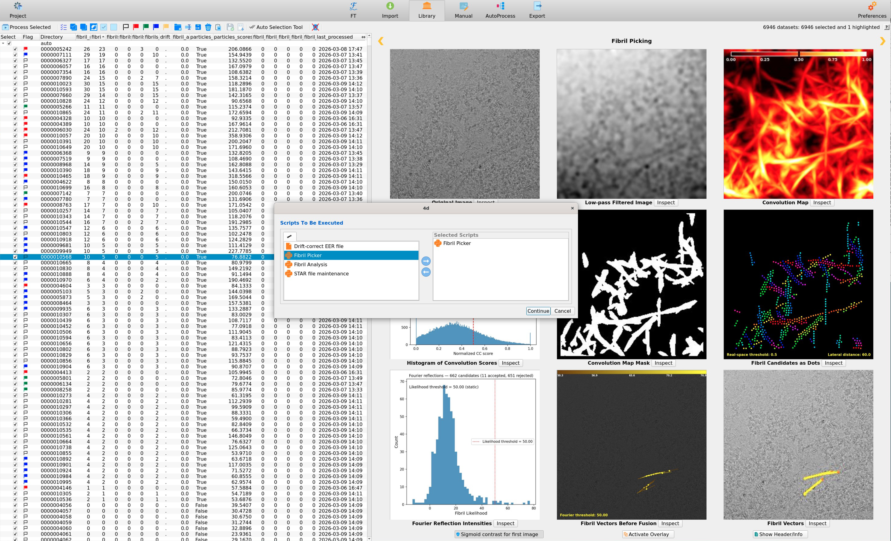
With the selection made, press Process Selected at the top-left of the Library toolbar. 4d then asks which scripts should run on those datasets, in the Scripts To Be Executed dialog:

Selecting the scripts to be executed on the selected datasets

Screenshot images/screenshot-fibril-launch.png not found — place it in the manual’s images/ directory.

1 2 3 4 5 6 7

#	Region	What it is
1	Library table	The datasets of the project, one per row. Every row's Select checkbox is ticked here — the whole session is selected.
2	Process Selected	The button that starts this step: it takes every ticked dataset and opens the script dialog. Disabled while nothing is selected.
3	Selection counter	“6946 datasets: 6946 selected and 1 highlighted” — confirm this before continuing.
4	Available scripts	The scripts of the current section — here the Fibrils scripts: Drift-correct, Fibril Picker, Fibril Analysis, STAR file maintenance.
5	Selected Scripts	What will actually run, in this order. Here only Fibril Picker — but several scripts can be chained, and each dataset then runs them in sequence.
6	→ / ← buttons	Move scripts between the two lists.
7	Continue	Submits the datasets, with those scripts, to the processing queue. Cancel aborts without queueing anything.

The scripts run with the parameters currently stored for each dataset — the same values you would see in the Manual tab. Establish your parameters on one or two representative datasets first, then submit the whole session here; there is no opportunity to adjust parameters once the queue is running.

Step 3 — The AutoProcess queue running

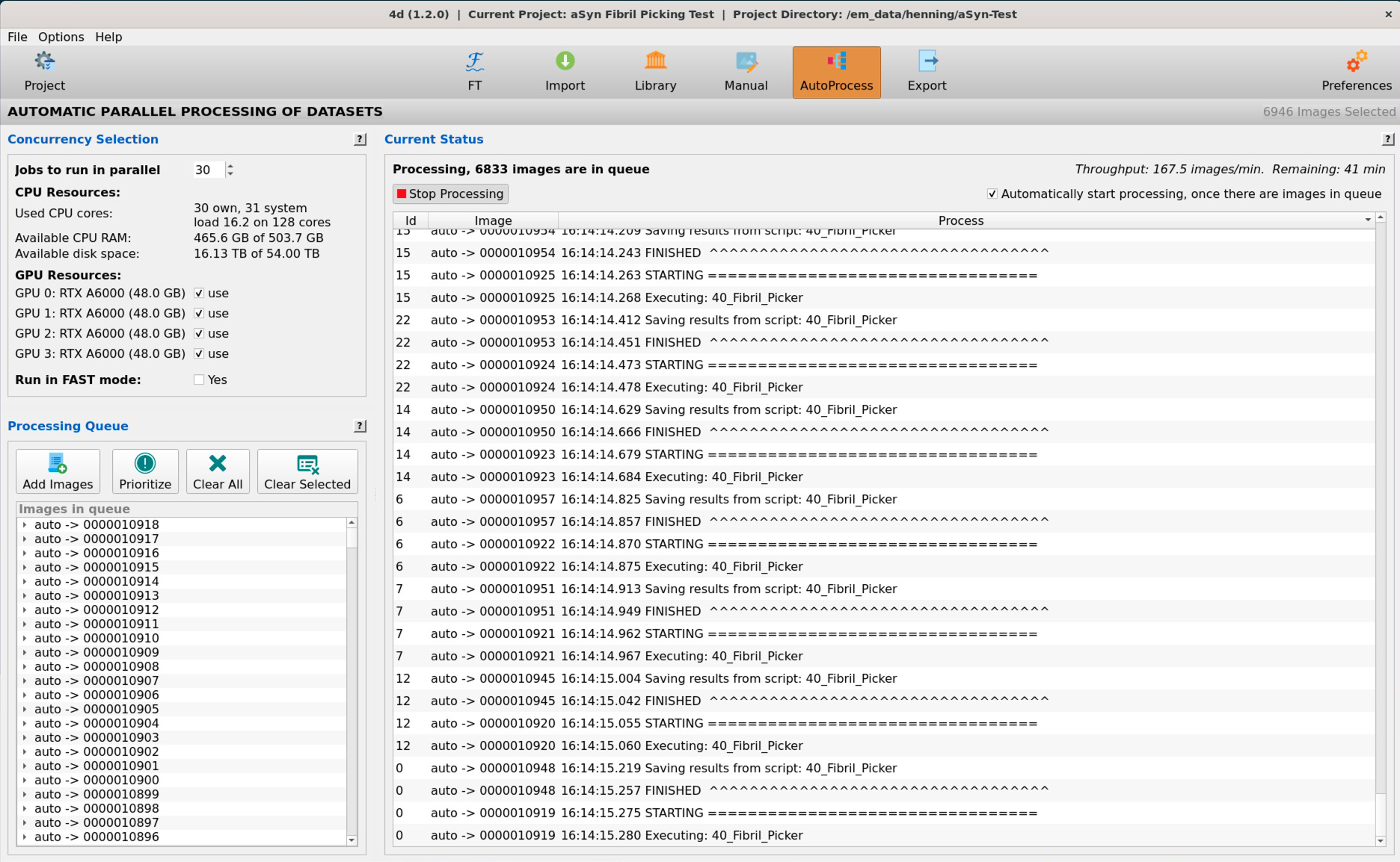
Pressing Continue hands the datasets to the AutoProcess tab, which runs them. The screenshot below is a real fibril-picking run on an Ubuntu Linux workstation, part-way through the queue:

The AutoProcess tab processing a large queue in parallel

Screenshot images/screenshot-fibril-throughput1.png not found — place it in the manual’s images/ directory.

1 2 3 4 5 6 7 8 9 10 11

#	Region	What it shows
1	Jobs to run in parallel	How many datasets are processed simultaneously — 30 here. This is the single most important performance setting; see Choosing the number of parallel jobs.
2	CPU / RAM / disk read-out	Live resource monitoring, refreshed every second: used cores (“30 own, 31 system”, load 16.2 on 128 cores), free RAM (465.6 GB of 503.7 GB) and free disk space. Watch the RAM figure — exhausting memory is the usual reason a high job count fails.
3	GPU Resources	The NVIDIA GPUs detected on the machine (four RTX A6000 here), each with a use checkbox so you can reserve one for other work. GPU-capable scripts distribute across the ticked GPUs; this section is absent on machines without NVIDIA GPUs.
4	Run in FAST mode	Sets the `fast_mode` parameter for every script; scripts that support it then skip their more expensive optional steps.
5	Processing Queue controls	Add Images (add the current Library selection to the queue), Prioritize (move highlighted queue entries to the front), Clear All and Clear Selected.
6	Images in queue	The waiting datasets, in the order they will be processed. Highlight entries here to Prioritize or Clear Selected them.
7	Stop Processing	Stops after the running jobs finish; everything still queued stays queued. Press again to resume.
8	Queue status	“Processing, 6833 images are in queue” — the live backlog, counting down as datasets finish.
9	Throughput & remaining time	167.5 images/min, Remaining: 41 min. The rate is measured over a sliding 60-second window, so it reflects the current speed rather than a long-run average — expect it to fluctuate during a run — and the remaining-time estimate follows it.
10	Automatically start processing	When ticked, the queue starts by itself as soon as datasets are added — combine it with continuous import for a fully hands-off pipeline that processes data as the microscope produces it.
11	Live log	One line per event per dataset: STARTING, Executing, Saving results, FINISHED. The Id column is the parallel slot, so you can follow one worker's progress through the interleaved output of all 30.

The worked example: 6900 micrographs in 45 minutes

The run shown above is fibril picking — the Fibril Picker script, including its full filter chain (binning, Hanning/Gaussian filtering, Kuwahara, bottom-hat, tubeness/Hessian scoring, and the per-candidate Fourier test) — on a complete session of about 6900 micrographs:

Quantity	Value
Machine	Ubuntu Linux workstation, 128 CPU cores, 512 GB RAM, 4 × RTX A6000
Parallel jobs	30
Throughput	≈ 150 images/min (the read-out fluctuates; 167.5/min at the moment shown)
Total	≈ 6900 images in ≈ 45 minutes

That is roughly 0.4 seconds per micrograph in wall-clock terms, although each individual micrograph takes on the order of ten seconds — the speed comes entirely from running 30 of them at once. Sequential processing of the same session would have taken most of a day.

The CPU read-out is worth a second look: 30 jobs, but a load average of 16.2 on a 128-core machine, and 465 GB of RAM still free. The machine is not saturated — this workload is limited by per-image work that does not parallelize inside a single job, so there is head-room here to raise the job count further. That is exactly the kind of judgement the live read-outs are there to support.

Throughput scales with the number of parallel jobs only as long as the machine can feed them. Verify the scaling on your own hardware: queue a few hundred datasets, read the throughput figure, adjust the job count, and watch how it responds.

Following progress in the Library

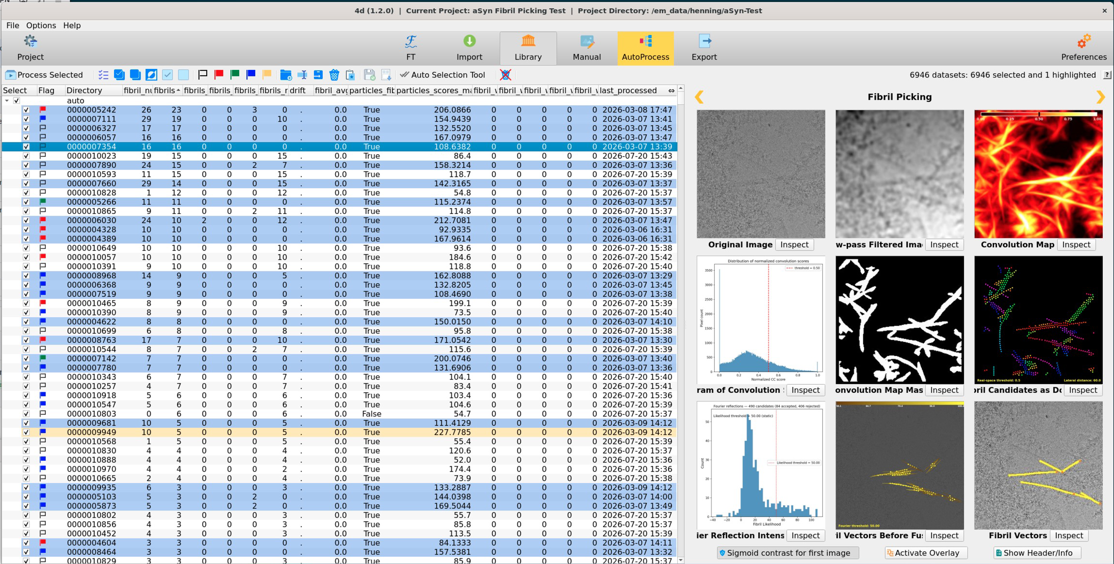
You do not have to stay in the AutoProcess tab. The Library table colours each dataset row by its processing state, so switching back gives an immediate overview of the whole session:

Row colour	State	Meaning
Blue	Queued	Submitted and waiting — the backlog still to be processed.
Yellow	Running	Currently being processed. These rows pulse gently between yellow and orange, so the active datasets are easy to spot. There are as many of them as you have parallel jobs.
White	Done	Finished (or never queued). The row's result columns are filled in with the values the scripts produced.

The Library table during processing, with queued, running and finished rows

Screenshot images/screenshot-fibril-throughput5.png not found — place it in the manual’s images/ directory.

1 2 3 4

#	Region	What it shows
1	Queued rows (blue)	Datasets waiting in the queue.
2	Running row (yellow)	A dataset currently being processed by one of the parallel jobs.
3	Finished rows (white)	Already processed — note their `last_processed` timestamps are from today's run, while the queued rows still show older dates.
4	Result columns filling in	As each dataset finishes, the values its scripts produced (fibril counts, scores, timestamps) appear in the table — sort by them to review the results while the rest of the queue is still running.

The AutoProcess button in the main toolbar also pulses yellow-orange while the queue is working, so you can tell processing is still running from any tab.

Choosing the number of parallel jobs

Jobs to run in parallel is capped at the number of CPU threads the machine reports, but the best value is usually lower than the maximum. Three limits decide it:

CPU. Each job is a separate process. Beyond roughly the core count they compete rather than add. Note that many Python/NumPy operations are themselves multi-threaded, so the load average is not simply the job count — compare the two read-outs rather than assuming.
RAM. Multiply one job's peak memory by the job count. Large micrographs or 4D-STEM stacks make this, not the CPU, the binding constraint. Watch the Available CPU RAM read-out during the first minutes of a run.
Disk. Many jobs reading and writing at once can saturate a slow disk or a network filesystem; on such storage a lower job count is often faster.

A practical approach: start at about half the core count, queue a few hundred datasets, and read the throughput figure. Raise the job count and watch whether throughput actually improves — when it stops improving, or RAM starts running low, you have found the machine's limit. The setting is remembered per project.

GPU-accelerated scripts need a different calculation: the limit is GPU memory, not system RAM, and too many concurrent jobs per GPU will fail with out-of-memory errors. Use the per-GPU use checkboxes to control which GPUs take part, and keep the job count modest for GPU workloads.

Practical notes

Stopping is safe. Stop Processing lets the running jobs finish and leaves the rest queued. Nothing is corrupted and nothing is lost — press it again to resume.
The queue can grow while it runs. Select more datasets in the Library and press Process Selected (or Add Images) at any time; they join the back of the queue.
Prioritize urgent datasets. Highlight entries in the queue list and press Prioritize to move them to the front — useful for checking a few representative datasets before committing to the rest.
Re-running is fine. Submitting a dataset again simply re-runs the scripts and overwrites the previous results with the current parameters.
Failures do not stop the queue. If a script fails on one dataset, that dataset is marked and the queue continues. Check its log in the Manual tab afterwards.
Combine with continuous import (Import tab) and Automatically start processing for a live pipeline: images are imported as the microscope writes them and processed immediately, so results are ready when the session ends.