1. What a 4D-STEM dataset isBack to top
In a scanning transmission electron microscope a small convergent electron probe is moved over the specimen in a raster. A conventional STEM detector integrates the scattered intensity into one number per probe position. A 4D-STEM experiment replaces that detector with a fast pixelated camera and stores the entire convergent-beam electron diffraction (CBED) pattern at every position. The result is a four-dimensional array: two real-space scan axes and two reciprocal-space detector axes.
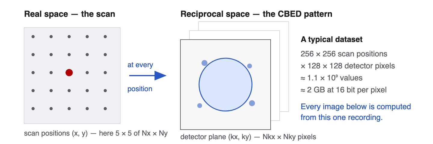
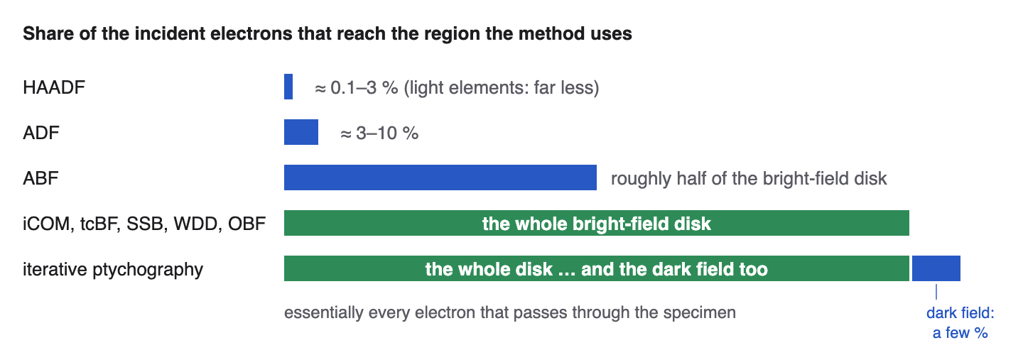
Two consequences run through everything that follows. First, nothing is thrown away at acquisition time: the choice of detector geometry becomes a processing parameter rather than a hardware decision. Second, the electrons are counted where they land, so methods that use the whole bright-field disk can be enormously more dose-efficient than a conventional annular detector that discards 95 % or more of them — the decisive argument for cryogenic and other beam-sensitive work.
2. The probe: focused and defocused illuminationBack to top
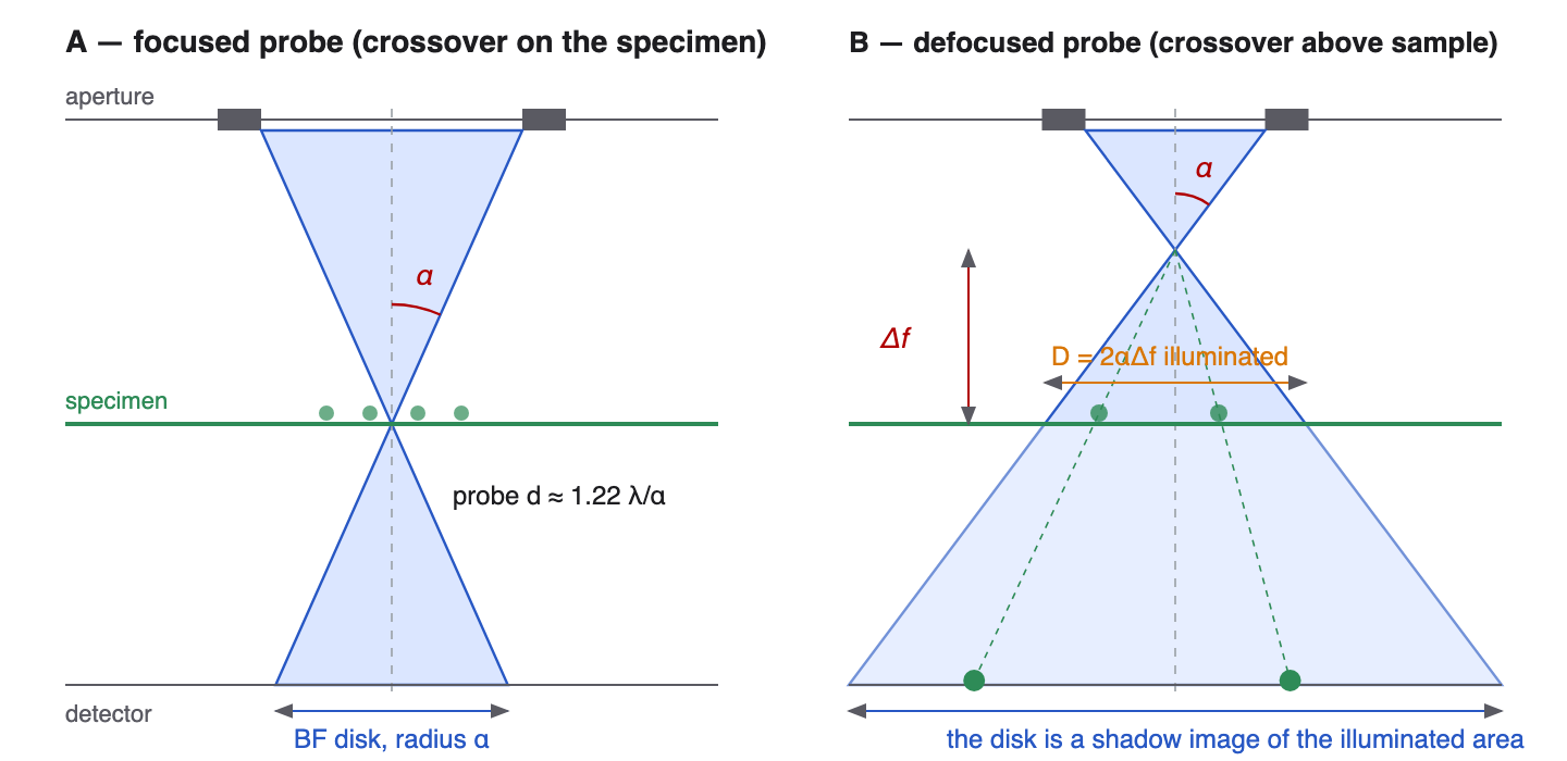
The illumination is a cone of semi-angle α, the convergence semi-angle (CSA), set by the condenser aperture. Where the cone's crossover sits relative to the specimen decides what a single CBED pattern looks like, and therefore which reconstruction algorithms make sense.
| Focused probe | Defocused probe | |
|---|---|---|
| Probe size | diffraction-limited, ≈ 1.22 λ/α (≈ 0.1 nm at 300 kV, α = 25 mrad) | D = 2αΔf (≈ 8 nm at α = 4 mrad, Δf = 1 µm) |
| Depth of field | ≈ 2λ/α², a few nm at large α — thick specimens are out of focus away from the focal plane | effectively the whole specimen; focus is recovered computationally |
| Dose per area | concentrated: high local dose rate | spread over a large area, so each position is dim but many positions overlap |
| Natural methods | ADF/HAADF, iDPC/iCOM, SSB, WDD, iterative ptychography | shadow imaging, parallax / tcBF, low-dose ptychography with large fields of view |
Both regimes need the scan step to be chosen with the probe size in mind. Phase-retrieval methods rely on neighbouring probes seeing the same object region: a typical requirement is 60–80 % overlap of the illuminated areas. Whether the step also sets the resolution depends on how the method uses each pattern, and the three cases behave quite differently:
- One number per scan position — virtual detectors (BF, ABF, DF, ADF, HAADF) and the raw CoM/DPC shift fields. The image grid is the scan raster, so the sampling limit k = 1/(2·step) applies literally.
- Solved on the scan grid — SSB and WDD, which Fourier-transform the dataset along the two scan axes. The recoverable spatial frequency is the smaller of the angular ceiling 2α/λ and the scan-sampling limit 1/(2·step), which is why focused-probe direct ptychography wants a step of roughly half the finest detail it is meant to resolve.
- Solved from the structure inside each pattern — shadow imaging, parallax/tcBF and iterative ptychography, and in particular anything run on a strongly defocused probe. Here the scan step does not set the resolution. One defocused pattern is already a magnified image of the illuminated patch, so the object is sampled at D/N, where N is the number of detector pixels across the bright-field disk: at α = 4 mrad and Δf = 1 µm the 8 nm patch read out over a disk a hundred pixels wide samples the specimen every 0.08 nm — far finer than any scan step one would use over a patch that size. The reconstruction is carried on that finer grid, and the ceiling is angular instead: (α + θmax)/λ for iterative ptychography, transfer towards 2α/λ for tcBF. What the step governs here is redundancy and freedom from periodic raster artefacts, not the finest detail that can be represented.
3. Virtual detectors: BF, ABF, DF, ADF, HAADFBack to top
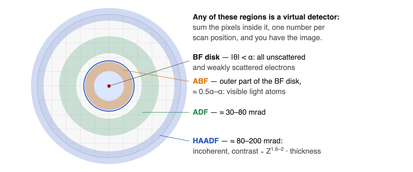
The simplest way to turn 4D data into an image is to add up the intensity inside a chosen region of the detector for each scan position — a virtual detector. This reproduces every classical STEM mode, and the regions can be changed and re-applied at will.
| Mode | What it measures | Strengths and limits |
|---|---|---|
| BF | Intensity inside (part of) the bright-field disk. With an axial pixel this is, by reciprocity, the equivalent of a conventional TEM bright-field image. | Phase contrast needs defocus, and the contrast transfer oscillates and changes sign. A large BF detector collects many electrons but averages contrast away; a small one has contrast but few electrons. |
| ABF | Annular bright field: the outer annulus of the BF disk, typically 0.5α–α. | Shows light atoms (O, N, Li, even H in favourable cases) next to heavy ones, which HAADF cannot. Contrast is not linear in the projected potential and depends on thickness and defocus. |
| DF / ADF | Electrons scattered outside the BF disk, at intermediate angles. | Mixes diffraction and mass-thickness contrast; strong for crystalline material, sensitive to orientation. |
| HAADF | Electrons scattered to high angles, dominated by thermal-diffuse (Rutherford-like) scattering. | Effectively incoherent: intensity rises monotonically with atomic number (≈ Z1.6–2) and thickness, no contrast reversals, directly interpretable. But only a tiny fraction of the electrons reach it, which makes it the least dose-efficient mode of all — unusable at cryogenic doses. |
4. DPC, CoM, iDPC and iCOMBack to top
A thin specimen barely absorbs electrons; it shifts their phase. In the ray picture, a local electric field — the field of the atoms themselves — deflects the probe slightly, and the whole bright-field disk moves sideways in the pattern. Measuring that displacement is differential phase contrast.
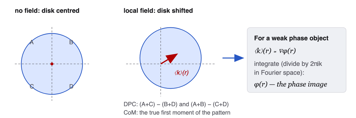
Why it is attractive: for a weak phase object the transfer is linear in the projected potential, so the image can be interpreted directly rather than matched against simulations; it uses the entire bright-field disk, so it is dose-efficient; and its transfer is strongest at low spatial frequencies, which is exactly where biological and other light-element contrast lives.
What to watch out for: the integration is a division by k in Fourier space, so noise and any slow instrumental drift at low spatial frequency are amplified into the familiar cloudy shading across iDPC images. A high-pass filter tames it (4d offers one directly next to the iDPC button) at the cost of removing genuine long-range signal. iDPC from quadrant detectors is also only an approximation of the first moment, and becomes non-linear for thicker specimens and strongly scattering (heavy, crystalline) material; iCOM from a pixelated detector is the more faithful measurement of the two.
5. Parallax / tcBF and shadow-image reconstructionBack to top
Parallax, also called tilt-corrected bright-field STEM (tcBF)
Reciprocity is the key idea: one pixel inside the bright-field disk is one illumination direction. Forming an image from a single BF pixel therefore gives a complete bright-field image of the scanned area, taken with the beam tilted by the angle of that pixel. A pixelated detector delivers hundreds or thousands of such images from one scan.
Because they are tilted views, defocus displaces them laterally by Δf·θ — the parallax that gives the method its name. The algorithm measures those shifts by cross-correlation, undoes them, and adds the images up.
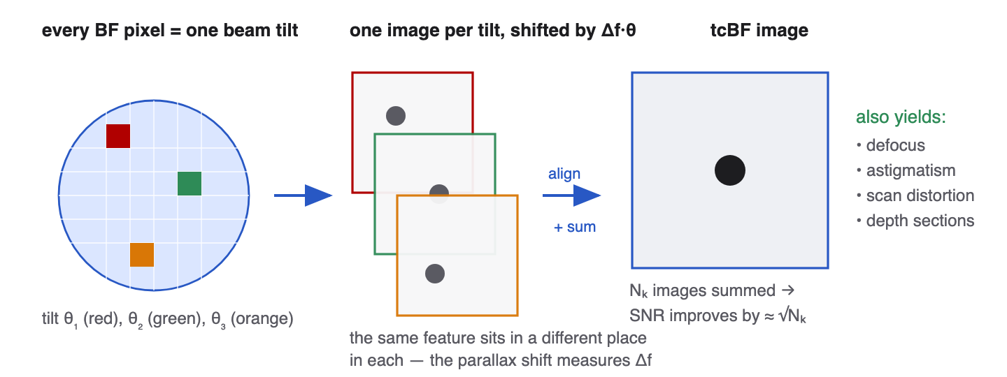
Two properties make tcBF attractive for thick, beam-sensitive specimens: the focus is set after the experiment, so the depth of field stops being a limitation, and the shift field can be refined per region, which corrects scan distortion and even allows optical depth sectioning by aligning for different heights.
What the alignment does not do is take the defocus out of the contrast transfer. For a tilt kt = θ/λ, the phase a spatial frequency q picks up is χ(kt + q) − χ(kt), and for defocus alone, χ(k) = πλΔf k², that splits into πλΔf q² + 2πλΔf kt·q. Only the second, linear term depends on the tilt — it is exactly the shift Δf·θ that the cross-correlation measures and removes. The first term is identical for every bright-field pixel, so no amount of shifting touches it. Each aligned view therefore still carries the phase-contrast transfer of a defocused lens, and so does their sum:
CTF(q) = A(q) · 2·sin χ(q), χ(q) = πλΔf q² + ½πCsλ³q⁴
— Scherzer's transfer function, oscillating through zeros and contrast reversals, not a monotonic incoherent-imaging envelope. A(q) is only the aperture term: the fraction of the disk that still overlaps itself at q, which does fall monotonically to zero at 2α/λ and sets the band limit. The oscillation sits inside that envelope, and it is fast: at 300 kV with Δf = 1 µm the first maximum of sin χ is near 20 Å and the first zero already at 14 Å.
What the alignment does buy is dose efficiency: the tilted views add coherently instead of washing one another out, so the sum has the counting statistics of the whole bright-field disk rather than of one pixel. Flattening the transfer is a separate step, and this is where the measured shift field earns its keep a second time — fitted for defocus, astigmatism and Cs, it gives the χ(q) that is then divided out of the summed image by a Wiener-like CTF correction. An uncorrected tcBF sum should be read as a defocused bright-field image, with all the interpretation problems that implies.
Shadow-image reconstruction
With a strongly defocused probe, Figure 2B, the same information appears directly in real space: each CBED disk is a small magnified image of the illuminated patch. Neighbouring probe positions image overlapping patches, so placing every disk on a common canvas at its scan position — scaled by a conversion factor and rotated to match the scan axes — stitches them into one large image. Where the scaling is correct the overlapping copies of a feature coincide and reinforce; where it is wrong they blur.
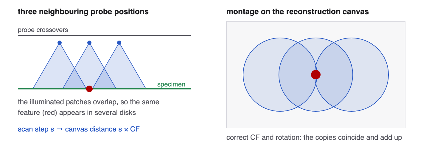
The montage does not change the contrast transfer, and it is worth being explicit about why. Seifer, Houben & Elbaum (2025) work the single disk out from Cowley's two-step propagation: for a weak phase object q = 1 + iφ illuminated through an aberration χ, the intensity recorded across the disk is
F{ |ψD|² } = 2A²·F{φ}·sin χ(k) + …
— so a single shadow image already carries sin χ, the same phase-contrast transfer as a wide-field TEM image taken at that defocus. Stitching does nothing to it: the defocus and the magnification are common to every patch, so every patch carries the identical sin χ(k), and the overlap-normalised average of many identical transfer functions is that same transfer function. The montage buys signal-to-noise and field of view, not a flatter CTF. That it lands on exactly the result of the tcBF paragraph above is no coincidence — the two are the same operation, and Seifer et al. show the montage is tcBF in the geometric-optics regime.
The first contrast reversal therefore sits at a spatial period √(λΔf): 1.6 nm at 200 kV and Δf = 1 µm, 1.4 nm at 300 kV, with reversals at every finer spacing, exactly as in wide-field TEM. Two things follow for practice. Keep Δf as small as the shadow regime allows — it must still exceed the depth of field λ/α², exceed ∼10·Csα² to hold the magnification non-linearity under 10 %, and exceed step/2α so the patches still overlap — and then correct the CTF by deconvolution. Seifer et al. frame the whole workflow as SSD: synchronisation (choosing CF and rotation), summation (the overlap), deconvolution (the CTF correction). 4d does the first two; the deconvolution is a downstream step, and it belongs on the assembled montage — correcting individual patches first introduces artefacts where they overlap.
One advantage over the wide-field TEM image it resembles survives all of this: because the focus is set by the probe and not by the objective lens, the shadow image is insensitive to energy loss in the specimen and to objective chromatic aberration — which is what makes the geometry attractive for thick, unfiltered cryo specimens in the first place.
6. Ptychography: SSB, WDD, OBF and iterative solversBack to top
Ptychography goes one step further than the methods above: instead of forming an image, it solves for the complex transmission function of the specimen from the redundancy in overlapping diffraction patterns. The family splits into direct (or analytical) methods, which compute the answer in one pass from a linear model, and iterative solvers, which refine object and probe until the computed patterns match the recorded ones.
That split is not only about how far each can reach, and it is worth knowing which side of it you want before acquiring anything. The direct methods are fast, need no starting guess, have essentially nothing to tune — no step size, no batch size, no loss and regularisation functions to balance — and cannot diverge, which also means they degrade predictably on sparse data with barely an electron per detector pixel, and give the same answer every time they are run. Those properties matter more than they sound. Low-dose work usually means repeating a measurement many times, and reproducibility across runs is what makes averaging or single-particle analysis downstream possible at all. The iterative solvers reach much further — past the aperture limit, through thick specimens, into partial coherence — but their answer depends on a parameter set, and different parameter sets give different answers.
The three direct methods — SSB, WDD and OBF — are not three different physical ideas. They are three inversions of one linear model, and it pays to write that model down once, because everything else follows from it. Fourier-transform the 4D dataset along the two scan axes. Each detector pixel K then reports, for each object spatial frequency Q,
G(K, Q) = |A(K)|²·δ(Q) + Φ(Q)·A(K)A*(K+Q) − Φ*(−Q)·A*(K)A(K−Q)
where Φ(Q) is the object's phase spectrum and A(K) = aperture × eiχ(K) is the probe in the detector plane, aperture and aberrations included. The first term is the unscattered disk; it sits at Q = 0 and carries no information about structure. The other two are interference between the direct beam and a beam scattered by ±Q — the two sidebands — and they are non-zero only where the bright-field disk overlaps a copy of itself shifted by ±Q. Every method below is a different answer to the same question: given those overlaps, how should the pixels be combined into an estimate of Φ(Q)?
Single-side-band (SSB) ptychography
SSB takes the simplest answer available: use only the pixels where exactly one sideband is present, because there the algebra collapses to something you can read off directly.
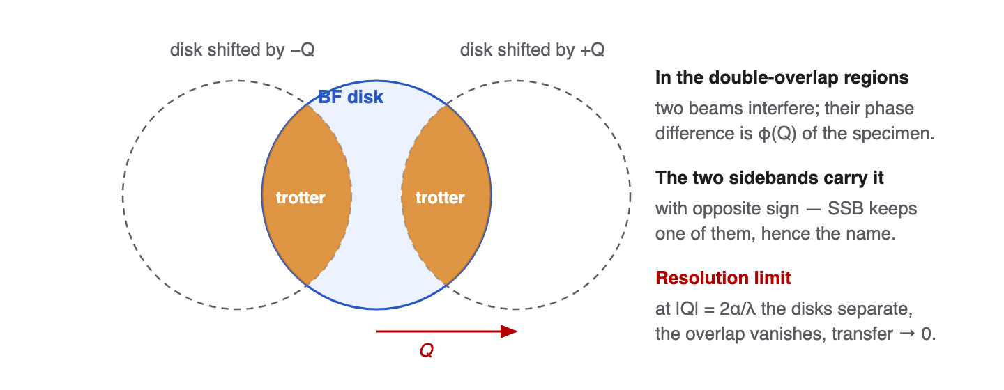
For a given Q, picture three disks — the bright-field disk and two copies of it shifted by +Q and −Q. Where the central disk overlaps the +Q copy but not the −Q copy, only one of the two interference terms survives. Those two crescent-shaped regions are the trotters, and inside them the recorded quantity is just
G(K, Q) = Φ(Q)·e i[χ(K) − χ(K+Q)]
— the object's phase at Q, rotated by a known amount. Two beams and only two reach such a pixel: the direct beam at K, and the beam the specimen scattered by Q. Their interference is the measurement, and since the aberration phase χ is known it can simply be divided out. Correct the pixels of one trotter, sum them, repeat for every Q, inverse-transform: the phase image drops out in a single pass. No starting guess, no iteration, nothing that can diverge.
Where all three disks overlap at once — the triple-overlap region in the middle — something sharper than ambiguity happens. The two sidebands are π out of phase with each other, so for an unaberrated probe they cancel exactly and the region transfers nothing at all. This is not a limitation of SSB; it is a property of the data, and it has a large consequence that §7 returns to — any detector that sums a centro-symmetric region, which is what plain BF and ABF detectors do, collects both anti-phase crescents together and cancels its own signal. SSB discards those pixels, and the second trotter with them: hence single side band. That is the method's one structural weakness. Something like half of the electrons that carry usable phase information are thrown away, which is exactly why SSB is beaten on noise by WDD and OBF, which use the same recording more completely.
One more property of the geometry is worth knowing, because it explains why the method tolerates an imperfect microscope. Along the line K = Q/2, halfway between the centre of the unscattered disk and the centre of the scattered one, χ(K) and χ(K−Q) are equal by symmetry, so all round aberrations cancel — spherical aberration included — without being known or corrected. The trotter phase is exactly right there and degrades smoothly away from it.
The transfer then follows from the geometry of the three disks alone:
- At Q = 0 the three disks coincide, the exclusive overlap has zero area, and there is no transfer at all. SSB is blind to the slowly varying part of the object — flat contrast, long-range mass-thickness — in the way a high-pass filter is.
- As Q grows the crescents open up and the transfer rises to a broad maximum.
- At Q = 2α/λ the shifted copies no longer touch the central disk, the overlap vanishes and the transfer returns to zero. That is the hard limit of every direct method that works from the bright-field disk alone (only WDD's dark-field "stepping out" mode, below, reaches past it) — and it is twice the conventional aperture limit α/λ, which is the classic reason for doing any of this.
Two practical consequences. Because χ enters the formula explicitly, SSB does not need a focused probe: it corrects the defocus as part of the inversion, and the defocus can be found by running the reconstruction over a range of values and keeping the sharpest result. And because the first step is a Fourier transform over the scan raster, the scan step imposes a ceiling 1/(2·step) on Q — §2 above — on top of the aperture limit.
Wigner-distribution deconvolution (WDD)
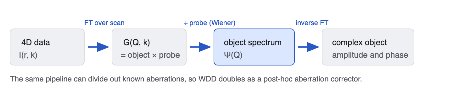
WDD inverts the same model, but instead of picking out the pixels where the algebra happens to be easy, it undoes the probe everywhere at once.
Put the 4D dataset through two transforms: Fourier over the scan coordinate R → Q as before, then inverse Fourier over the detector coordinate K → ρ. In this mixed domain — one reciprocal axis, one real axis, which is what makes it a Wigner representation — the convolution that ties probe and object together becomes a plain product:
H(Q, ρ) = Wprobe(Q, ρ) · Wobject(Q, ρ)
and a product can be divided. The probe term is computed from the aperture and the known aberrations, so dividing it out leaves the object term, from which Φ(Q) is read and inverse-transformed into the image.
The division is where the care goes. Wprobe has zeros and near-zeros, and dividing by a small number multiplies whatever noise sits there by a large one. So the division is done as a Wiener filter, W*/(|W|² + ε): where the probe transfers well this is an honest division, and where it does not, the ε quietly caps the gain. That single number is the method's main knob and it is a direct trade — a small ε buys resolution and pays in noise, a large one the other way about.
What the deconvolution buys over SSB is the use of all the interference: both sidebands, triple-overlap region included. The dose is used far better, and the transfer comes out approximately flat up to 2α/λ instead of collapsing to zero at low Q, so unlike SSB it keeps the long-range contrast. It also recovers the modulus of the transmission function alongside its phase, which lets absorption and phase be looked at separately. What it costs is knowledge: the probe model has to be right, and a wrong aperture size or an unmeasured astigmatism shows up as a systematic artefact rather than as extra noise. It is also the most memory-hungry of the direct methods, since it transforms the full 4D array along both pairs of axes.
One further capability sets WDD apart from the other two. The deconvolution can be continued outside the bright-field disk — the "stepping out" approach — relating the intensity scattered beyond the primary beam to the object frequencies lying past 2α/λ. WDD can therefore reach spatial frequencies SSB and iCOM cannot, and it is the one place a direct method crosses the aperture limit. The catch is that this needs a useful number of electrons out in the dark field, and for a weak phase object there are very few: the technique is expensive in dose, and belongs to radiation-hard specimens rather than cryogenic ones.
Optimum bright field (OBF)
OBF starts from the same linear model but asks a statistical question rather than an algebraic one: given that every bright-field pixel carries some information about Φ(Q), and that each of them also carries Poisson noise, what is the best possible way to combine them?
Write the image formed from detector pixel K alone as GK(Q) = βK(Q)·Φ(Q) + noise, where βK(Q) is that pixel's own transfer — the same overlap-and-aberration factor as in the model above, computable as soon as the aperture and the aberrations are known. The estimator with the highest signal-to-noise ratio is then the classic matched filter:
ΦOBF(Q) = ΣK β*K(Q)·GK(Q) / ( ΣK |βK(Q)|² + ε )
Each pixel is weighted by exactly how much signal it actually carries at that frequency, and pixels that carry none get no weight — instead of being summed in blindly, as a plain bright-field detector does (which is why its contrast partly cancels), or discarded wholesale, as SSB does with its second trotter and its triple overlap. The result is the best signal-to-noise ratio any linear estimator can reach for a weak phase object at a given dose and aperture. That is what the word "optimum" is claiming, and within the model it is a provable claim rather than a comparative one.
In practice OBF produces images that look much like SSB, with visibly less noise and with the low frequencies restored. Two further properties matter at the microscope. First, the weighting can be recast as a small set of real-space filters applied to the bright-field images, so OBF can run live during the scan, frame by frame, without storing or re-reading the 4D dataset — which is why it has become the usual "watch the phase while you acquire" mode. Second, it degrades gently when the object is not really weak: it remains a weighted sum of genuine bright-field images, so it drifts towards an ordinary, mildly non-linear phase-contrast image instead of breaking down.
Iterative ptychography and ePIE
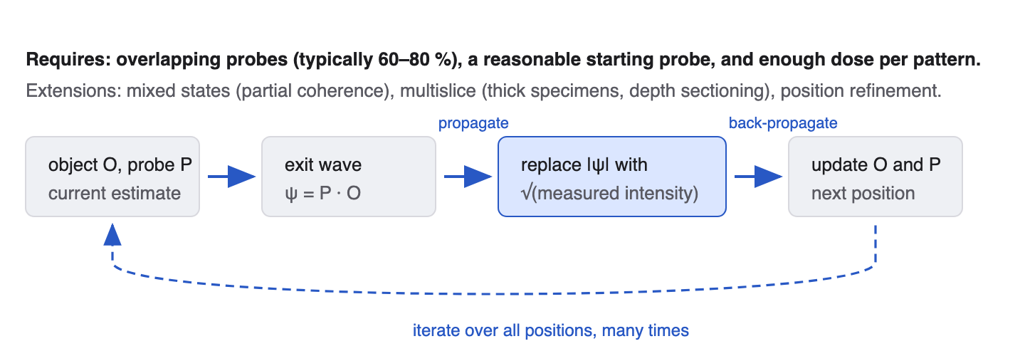
Iterative solvers make no weak-object assumption. They maintain estimates of both the object and the probe, simulate the pattern each scan position should produce, and correct the estimates wherever the simulation disagrees with the measurement — over and over, using the overlap between neighbouring positions as the constraint that ties everything together. The family is much easier to follow once the loop is written out, so it is worth doing once.
The forward model, and the one trick everything rests on
Single-slice ptychography assumes the exit wave at probe position Rm is a plain product of illumination and object:
ψm(r) = P(r)·O(r − Rm), Jm(k) = | F[ψm(r)] |²
with Jm the pattern the current estimate predicts and Im the one actually recorded. The solver minimises the mismatch between them, typically E = Σm,k (√Im − √Jm)². What makes this tractable is that the minimal change to a complex exit wave that forces it to agree with a measured intensity is obvious: keep its Fourier phase, and replace its Fourier amplitude with the square root of what the camera saw.
ΠF[ψm] = F−1[ √Im(k) · F[ψm] / √Jm(k) ]
That is the Fourier projection, and it is the only place the measurement enters. Everything else in the loop is bookkeeping about how to push the resulting correction Δψm = ΠF[ψm] − ψm back onto the object and the probe:
O′ = O + β·||P||α−1 Σm∈M P*·Δψm, P′ = P + β·||O||α−1 Σm∈M O*·Δψm
Here β is the step size and α sets how the update is normalised. ePIE — the extended ptychographic iterative engine, the algorithm most people mean by "iterative ptychography" — is exactly this loop with the batch M reduced to a single probe position: update object and probe, step to the next position, repeat. Take larger batches and it becomes stochastic gradient descent; take every position at once and it becomes plain gradient descent. Seen that way ePIE is not a separate invention but one end of a continuum, and the continuum is where the practical guidance lives:
- Batch size. Large batches — as many positions as memory allows — are both more accurate and computationally more efficient. Small batches, ePIE's limit, converge the probe faster, which matters whenever the probe is being solved for as well, mixed-state reconstructions above all.
- Normalisation α. For clean high-dose data α → 0 reaches the lowest error; for low-dose experimental data α → 1 is almost always better behaved. It is one of the few hyper-parameters worth setting deliberately rather than leaving at a default.
- Relatives. Replace the gradient step with a projection between constraint sets and a whole named family appears — alternating projections (the classical "error reduction", and nearly identical to gradient descent at β = 1), difference map, RAAR, RRR. Difference map tends to diverge on electron data; its relaxed variants RAAR and RRR behave considerably better. Because they are all points in one parameter space, they can be, and increasingly are, tuned per dataset by Bayesian optimisation against a reconstruction-quality metric.
What it buys, and what it demands in return
Two advantages are structural. Probe and object are solved together, so residual aberrations stop being a resolution limit — the solver absorbs them into the probe. And the reconstruction is carried on a grid set by the largest recorded scattering angle, Δx = 1/(2kmax), not by the scan step. That is the formal statement of the super-resolution discussed in §2: the detector sets the resolution, the scan step only sets the redundancy.
Which explains a habit that looks wrong at first sight. Defocus is often introduced deliberately before a ptychographic acquisition: a larger probe overlaps its neighbours more, giving more redundancy per electron, which permits a coarser scan and a faster acquisition at the same dose. Around 70–80 % overlap is the usual target. Buying it with defocus costs reconstruction array size; buying it by shrinking α changes the transfer instead (§7).
The demands are equally concrete. These solvers can converge on a wrong answer, and in practice they are kept honest by constraints rather than by good luck:
- On the object — storing it as eiV with a real potential V, rather than as a free complex array, halves the memory and lets physical priors be imposed directly: atomic potentials are non-negative, so negative values can be clipped, and a shrinkage filter that subtracts a constant phase before clipping drives the background to zero and promotes atomicity.
- On the probe — a fixed aperture taken from a real vacuum measurement, a smooth aberration surface, centre-of-mass fixing. A good vacuum probe is the single most valuable calibration in the whole workflow: without it object detail leaks into the Fourier amplitude of the probe (probe–object mixing), and constraining the aperture removes half the solution space at a stroke.
- On the positions — refining the scan positions over the first hundred or so iterations absorbs sample drift and scan distortion, which otherwise appear as a blur that no amount of further iteration removes.
Mixed-state ptychography: when one probe is not enough
Everything above assumes a perfectly coherent probe. Real illumination never is — finite source size and energy spread make it partially coherent — and a single-state solver handles the mismatch by dumping the discrepancy into the object, which quietly degrades everything. The fix is to represent the illumination as several mutually incoherent probe modes and to add their intensities, not their amplitudes:
ψm(l) = P(l)(r)·O(r − Rm), Jm(k) = Σl | F[ψm(l)] |²
The modes must be re-orthogonalised at every iteration, because nothing in the update itself keeps them independent. The payoff is large and well documented: treating partial coherence properly is a prerequisite for reconstructions that are simultaneously high-resolution, precise and wide-field, and measured against conventional atomic-resolution STEM the mixed-state approach has delivered four-times-faster acquisition with double the information limit at the same dose — or the same resolution at up to fifty times less dose. It is also where small batches earn their keep, since the probe modes need that faster probe convergence.
7. CTF, noise, SNR and doseBack to top
Almost all the phase-imaging methods can be compared on the same footing, because for a weak phase object each of them is linear: the image spectrum is the object phase spectrum multiplied by a contrast transfer function CTF(k). Two numbers then decide how a method performs at a given dose — how large |CTF(k)| is at the frequencies you care about, and how many of the incident electrons the method actually uses. (Iterative ptychography is the exception: it is non-linear, and the curve drawn for it below is an effective transfer measured from a reconstruction, not a filter the method applies.)
The single most useful thing to know about a method's CTF(k) is whether it oscillates. A transfer that changes sign has zeros, and at a zero the corresponding feature size is simply absent from the image; on the far side of it the contrast is reversed, so atoms that were dark become bright. Methods whose contrast still originates in a defocused lens — a plain defocused bright-field image, and with it tcBF and the shadow montage — all inherit sin χ(k) and therefore all have an oscillating CTF and need a CTF correction before their densities can be read quantitatively. The need for CTF correction is what distinguishes them from the phase-retrieval methods. The phase-retrieval methods, in contrast, have a single-signed CTF — one that never crosses zero, even where, as with SSB's band-pass, it rises to a maximum and falls again — so they do not require CTF correction. In particular, the phase-retrieval methods that solve for Φ(Q) directly (iDPC/iCOM, SSB, WDD, OBF) do not oscillate: their transfer is single-signed, so what is dark is dark everywhere it is resolved at all.
The transfer ceiling, and why it has the shape it has
There is a single curve that every method in this document is measured against. For a weak phase object imaged with an unaberrated probe, the transfer available to any detector is proportional to the area of the double-overlap regions — the trotters of §6 — and that area has a closed form. Writing ω = Q/α for the spatial frequency in units of the convergence semi-angle, and with a(u) = cos−1(u) − u√(1−u²) the half-area of the lens-shaped overlap of two unit disks a distance 2u apart,
CTF(ω) ∝ 4·a(ω/2) − 4·a(ω) for ω ≤ 1, 4·a(ω/2) for 1 < ω ≤ 2
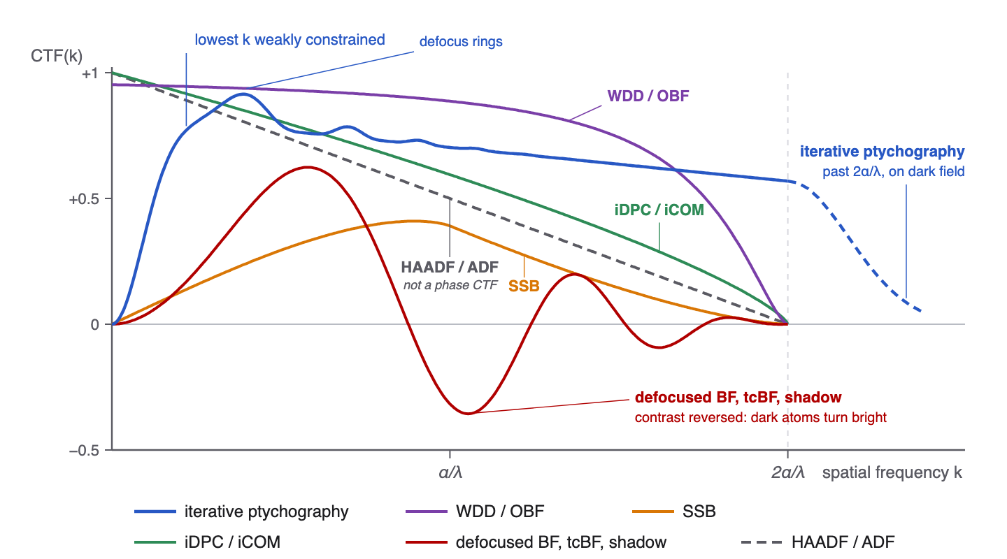
The first term is the full overlap of the shifted disks, the second subtracts the triple overlap that cancels. Three things follow, and they are the reason the orange curve in Figure 10 looks the way it does: the transfer is zero at ω = 0 and zero at ω = 2, and in between it peaks at ω ≈ 0.9 — that is, at a spatial frequency of about 0.9α/λ.
Why a bright-field detector sees nothing — unless you defocus it
The same geometry explains a result that surprises people. The two trotters are π out of phase with one another, so their intensities vary in anti-phase as the probe moves. A detector that integrates a centro-symmetric region therefore collects both and they cancel: BF and ABF detectors have exactly zero contrast transfer for a weak phase object with an unaberrated probe. What contrast they do show comes from somewhere else entirely — from defocus and spherical aberration breaking the symmetry, or from multiple scattering and channelling in a thicker specimen. It is why an ABF image of bilayer graphene taken with an in-focus aberration-corrected probe is very nearly blank, while a ptychographic reconstruction of the same scan is sharp; and it is the deeper reason the table below qualifies BF with "only with defocus".
How finely must the disk be sampled?
Pixel size matters for a reason that also follows from the anti-phase argument: a detector pixel large enough to straddle two anti-phase regions cancels part of its own signal. So transfer improves as pixels shrink, but it saturates, and it saturates early. Measured as peak SNR of a reconstructed single carbon atom, the curve plateaus at about 16 × 16 pixels across the bright-field disk, with 8 × 8 often good enough — useful to know, because fewer pixels means a faster camera and leaves the rest of the detector free to record dark field at the same time. Three pixels is the theoretical minimum for the reconstruction to work at all.
That number is a focused-probe result, and it does not carry over to defocused 4D-STEM — which matters, because that is the regime §5 and most of the cryogenic work above live in. With a focused probe the structure inside the bright-field disk is the overlap geometry, whose angular scale is α; a pixel only has to be small enough not to straddle two anti-phase regions, and a couple of dozen across the disk manage that however the experiment is set up. With a defocused probe the disk is a shadow image, so its pixels are no longer counting interference regions — they are sampling a picture, and the requirement becomes Nyquist on that picture:
N ≥ D/Δx = 2αΔf/Δx
with N the pixels across the disk, D = 2αΔf the illuminated patch and Δx the sampling wanted. Note what is not in that expression. The disk subtends 2α whatever the defocus, so defocusing never gives you more pixels — it packs more specimen area into the same ones. Sampling the shadow at its own optical limit λ/2α therefore needs
N ≥ 4Δf / (λ/α²)
— four pixels for every depth of field of defocus. Since the shadow regime already requires Δf to exceed the depth of field several times over, this lands in the tens and hundreds rather than the teens. The cryo-ptychography conditions quoted earlier — α = 1.03 mrad, Δf = −13 µm at 300 kV — sit at seven depths of field, so they need about 28 pixels across the disk merely to reach λ/2α ≈ 1 nm, and about 270 to sample that 26.9 nm patch at 1 Å. Which is why such experiments run on 256 × 256 cameras with the camera length set to spread the bright-field disk across a good fraction of the sensor. A 16 × 16 detector, ample for focused-probe SSB, would be useless for them. Iterative ptychography states the same condition from its own side: the reconstruction window is 1/Δk and it has to contain the probe, which is Δk ≤ 1/D again. With one important difference: 4Δf/(λ/α²) is the number at which the window equals the probe, and a window merely equal to the probe wraps around. A ptychographic reconstruction wants roughly twice that, so the window comfortably contains the illumination.
A worked case: which detector for low-dose cryo ptychography?
Put numbers on it, at 300 kV (λ = 1.97 pm) across the convergence angles and the two defoci a cryo experiment would realistically choose between. The column that decides everything is the last one, and it carries two numbers:
- The minimum is 4Δf/(λ/α²), the count at which the reconstruction window 1/Δk exactly equals the illuminated patch D. At that point the probe fills the window edge to edge, so anything it scatters wraps around and re-enters on the far side. It is a floor, not a target: a reconstruction run there is already corrupted.
- The wanted figure is twice the minimum, which makes the window about twice the probe and leaves the illumination surrounded by empty canvas. This is the number to design to.
| CSA α |
resolution λ/2α for 300kV |
depth of field λ/α² | Δf | patch D = 2αΔf | Δf in depths of field | px across the disk minimum (window = probe) / wanted (window = 2 × probe) |
|---|---|---|---|---|---|---|
| 1 mrad | 9.85 Å | 1970 nm | 500 nm | 1 nm | 0.3 | 1 / 2 |
| 1 µm | 2 nm | 0.5 | 2 / 4 | |||
| 2 mrad | 4.92 Å | 493 nm | 500 nm | 2 nm | 1.0 | 4 / 8 — but see below |
| 1 µm | 4 nm | 2.0 | 8 / 16 | |||
| 3 mrad | 3.28 Å | 219 nm | 500 nm | 3 nm | 2.3 | 9 / 18 |
| 1 µm | 6 nm | 4.6 | 18 / 37 | |||
| 4 mrad | 2.46 Å | 123 nm | 500 nm | 4 nm | 4.1 | 16 / 33 |
| 1 µm | 8 nm | 8.1 | 32 / 65 | |||
| 5 mrad | 1.97 Å | 79 nm | 500 nm | 5 nm | 6.3 | 25 / 51 |
| 1 µm | 10 nm | 12.7 | 51 / 102 | |||
| 6 mrad | 1.64 Å | 55 nm | 500 nm | 6 nm | 9.1 | 37 / 73 |
| 1 µm | 12 nm | 18.3 | 73 / 146 | |||
| 7 mrad | 1.41 Å | 40 nm | 500 nm | 7 nm | 12.4 | 50 / 99 |
| 1 µm | 14 nm | 24.9 | 99 / 199 | |||
| 8 mrad | 1.23 Å | 31 nm | 500 nm | 8 nm | 16.2 | 65 / 130 |
| 1 µm | 16 nm | 32.5 | 130 / 260 |
The shadow regime needs Δf to exceed the depth of field, and at 2 mrad the depth of field is 493 nm — so 500 nm of defocus is one depth of field and the probe is still essentially focused, with the shadow picture not yet applying. The defocus criterion returns 4 pixels there, which is meaningless; what governs instead is the focused-probe plateau from earlier in this section, 16 pixels across the disk. Only past about two depths of field does the defocus requirement overtake that floor and become the number that matters.
Both ends of the table are governed by the same scaling: the depth of field goes as 1/α², so the 1 µm of defocus that is two depths of field at 2 mrad is eight at 4 mrad and thirty-two at 8, and the pixel count follows it. Small angles struggle to reach the shadow regime at all; large ones reach it so emphatically that the detector cannot keep up.
Now the dose, and this is where the choice is really made. Take 10 e−/Ų with a 1 nm scan step — a realistic cryogenic budget. Each pattern then receives dose × step² = 1000 electrons, and spread over the bright-field disk that is
| sensor | px in the BF disk | electrons per pixel |
|---|---|---|
| 64 × 64 | 804 | 1.24 |
| 96 × 96 (ARINA binned) | 1810 | 0.55 |
| 128 × 128 | 3217 | 0.31 |
| 192 × 192 (ARINA) | 7238 | 0.14 |
| 256 × 256 | 12868 | 0.08 |
| 512 × 512 | 51472 | 0.019 |
| 1024 × 1024 | 205887 | 0.0049 |
Every one of these is in the sparse regime, where most pixels are empty and the pattern is a list of single-electron events rather than an image. That is not fatal in itself — a counting or event-driven direct detector records single electrons faithfully, and the analytical methods of §6 are built for exactly this, handling sparse patterns without any risk of diverging. But it is not free either: iterative solvers become markedly less stable below roughly an electron per pixel, and a larger sensor reads out more slowly, which costs scan positions and therefore field of view at fixed drift.
The decisive point is what the extra pixels actually buy. With the disk on half the sensor the reconstruction pixel is Δx = λ/4α — 123 pm here — whatever the sensor size. A bigger sensor does not buy resolution; it buys a larger reconstruction window per pattern, and it pays for that in electrons per pixel and in readout speed. At 10 e−/Ų that is a bad trade unless the window is genuinely needed.
Step up to 128 × 128 when you need Δf = 1 µm (an 8 nm patch will not fit the smaller window) or when the probe is aberrated enough to want the room. It costs a factor of four in electrons per pixel, down to 0.31, which analytical reconstruction tolerates and iterative solvers may not. Going to 8 mrad forces 256 or 512 and drops below 0.1 e−/px while buying a finer grid there are no electrons to fill; going below 64 × 64 stops the illumination fitting in the window at all.
Shape matters as well as size. Tri-sector and quadrant detectors produce transfer functions with three- and four-fold symmetry, which can interfere awkwardly with a crystal of similar symmetry; a 4 × 4 square array is already nearly circularly symmetric. And a 4-ring, 16-segment DPC detector transfers less than a 4 × 4 array of the same 16 pixels, because each of its segments spans a wider angular range and so is more likely to collect anti-phase signal. Conversely, running a ptychographic inversion on data from a plain quadrant DPC detector gives a markedly better SNR than forming the DPC difference signals from the same data — the inversion is worth doing even when the detector is coarse. These too are focused-probe statements: a segmented detector cannot do defocused work at all, however its signals are weighted, because a shadow image cannot be assembled out of four quadrants.
Choosing the convergence angle
Because the transfer peaks at ω ≈ 0.9, the convergence angle is not a fixed property of the microscope but a free parameter to be matched to the specimen. Place 0.9α/λ on the spatial frequencies that carry the structure of interest. For biological material, whose information sits at low spatial frequencies, this means deliberately reducing α, even on an aberration-corrected instrument: to put the transfer maximum at a 0.48 nm spacing at 80 kV, the convergence angle wanted is around 8.7 mrad, not the 30 mrad or more a corrected probe makes available.
Worth doing once as arithmetic, because the rule is short. The transfer peaks at ω = Qλ/α ≈ 0.9, so for a target spacing d the convergence angle wanted is α ≈ λ/(0.9 d). At 300 kV (λ = 1.97 pm) aiming at 3 Å, that is 7.3 mrad. (The 8.7 mrad quoted just above follows the slightly rounder α = λ/d convention of the original paper, which here would give 6.6 mrad; the two bracket the useful range.)
What the choice is worth is easy to underestimate. At 7.3 mrad the transfer at 3 Å is at its maximum by construction. At 10 mrad it is still 88 % of that. But at 4 mrad — an entirely reasonable-looking cryo setting — 3 Å sits at ω = 1.64, far down the falling flank, and the transfer is only 22 % of peak. The aperture limit is not the problem: 2α/λ at 4 mrad is 2.5 Å, so 3 Å is comfortably inside the band. It is simply being transferred badly. A factor of four and a half in contrast, for free, from one lens setting.
Now bring the defocus in, because the two choices are not independent. At 7.3 mrad the depth of field is only λ/α² = 37 nm, so the Δf = 1 µm of the question is twenty-seven depths of field. That illuminates a 14.6 nm patch and, by the rule of the previous section, needs about 216 pixels across the bright-field disk — a 512 × 512 sensor. Drop the defocus to 300 nm and the same 7.3 mrad probe illuminates 4.4 nm, sits at eight depths of field, and needs 65 pixels across the disk: a 128 × 128 detector, with all the speed and counting statistics that brings. The order to decide in is therefore: the resolution target fixes α; the detector then fixes how much defocus you can afford, not the other way round.
Cryogenic work pushes this much further. A virus particle 50–100 nm across has the spatial frequencies that define its shape at 0.01–0.02 nm−1, and a 1 mrad probe transfers that range far more efficiently than a 5 or 10 mrad one. The published cryo-ptychography of rotavirus and HIV-1 particles was accordingly recorded at 300 kV with α = 1.03 mrad and Δf = −13.0 µm — which by D = 2αΔf is a 26.9 nm probe, squarely in the defocused regime of §2 and Figure 2B. The three chapters meet here: the convergence angle sets where the transfer peaks, the defocus sets how large the illuminated patch is, and together they decide both what the method can see and how the electrons are spread over it.
The CTF of an iterative reconstruction is a property of the algorithm
Everything above is the transfer of a linear inversion, computable in advance from the optics. Iterative ptychography has no such closed form: the phase is reconstructed in silico, so the algorithm and its regularisation control the resulting information transfer, and they also impose an implicit, frequency-dependent noise filtering. Its CTF is therefore something you measure — reconstruct a known weak phase object and read off the transfer — which is exactly what the blue curve in Figure 10 represents.
It is worth separating two things that are easy to conflate. The transfer of a converged, noise-free ptychographic reconstruction is flat — CTF(k) ≈ 1 at every frequency the data constrain, including beyond the diffraction limit, with only the very lowest frequencies lagging because they need many iterations to converge. What is not flat is the signal-to-noise ratio at finite dose, and that is where the defocus of the recorded dataset reappears: certain frequencies come back with a markedly lower random error, in a Thon-ring pattern that follows the parallax transfer sin χ but is much sharper — close to its fourth power. Those are the ripples on the blue curve in Figure 10, and they matter in practice, because they are strongest below α/λ, exactly where a defocused acquisition is usually aimed. Unlike the zeros of a genuine sin χ CTF they never reach zero, so no spacing is lost — only unevenly favoured.
Measured that way, the headline property is the absence of zero crossings. A ptychographic power spectrum is continuous and shows no Thon rings, where a conventional defocused TEM image of the same specimen is crossed by them; there are no contrast reversals anywhere in the band, and the transfer at low spatial frequency is better than defocused TEM achieves, not worse. That combination is why cryo-ptychography can work at doses like 22.8 e−/Ų on rotavirus particles and 5.7 e−/Ų on HIV-1 virus-like particles while still resolving capsid features — conventional cryo-EM buys its low-frequency contrast with a large defocus and pays for it in rapid CTF oscillation at everything finer.
First, CTF(k) and dose efficiency are different quantities, and the SNR expression below keeps them in different factors: |CTF(k)| says what fraction of the object's signal at that frequency survives into the image, while η says what fraction of the incident electrons contributed at all. A method can score well on the first and catastrophically on the second. HAADF is exactly that case: for a weak phase object almost nothing scatters to high angle, so η is a per cent or less, and no amount of transfer rescues an image built from two electrons per pixel.
Second, and more fundamentally, the grey curve is not a phase CTF. HAADF is incoherent and scales as Z1.6–2; what is plotted for it is the transfer of scattering power, not of phase. It shares an axis with the others only for shape comparison, which is why it is dashed. For a vitrified biological specimen the honest statement is the one in the dose table above — HAADF and ADF are essentially blank — and the red curve, for all its reversals, is carrying real signal where the grey one is carrying almost none.
How many electrons does a method actually use?
Noise and SNR
Electron counting is Poissonian, so with N electrons per resolution element the relative noise is 1/√N. Combining that with the transfer function gives the practical rule of thumb for a weak phase object:
SNR(k) ≈ 2·φ(k)·|CTF(k)|·√(η·D·A)
with φ(k) the object phase at that frequency, D the dose in e−/Ų, A the area of a resolution element, and η the fraction of electrons the method uses (Figure 11), including the detector's own efficiency (DQE). Three practical consequences:
- SNR grows only as the square root of dose. Four times the dose buys twice the SNR. For beam-sensitive specimens the dose is capped by radiation damage, so the only free parameters are η and |CTF(k)| — which is precisely what the choice of method controls.
- Noise is shaped by the algorithm. iDPC/iCOM integrate, which is a division by k: low-frequency noise and drift are amplified into slow shading. SSB throws away both the second sideband and the triple-overlap region, so it works with roughly half the informative electrons and gives away about √2 in SNR against methods that use all of them. WDD and OBF apply a Wiener-like weighting that is optimal under their assumptions — OBF is explicitly derived to maximise SNR, and its advantage over SSB is largest at low spatial frequency, where SSB has no transfer to be noisy about in the first place. A defocused BF, tcBF or shadow image is a separate case again: its noise is unremarkable, but its zeros destroy information outright, and no amount of dose brings back a spacing that fell on one. Iterative solvers are non-linear, so their noise cannot be written as a filter at all: at low dose they need regularisation, and unregularised runs happily fit noise.
- Dose fractionation matters. For a fixed total dose, a finer scan step spreads the electrons over more patterns; each pattern is noisier but there are more of them, and phase-retrieval methods exploit the resulting redundancy. Below roughly ten electrons per pattern, direct methods stay well behaved while iterative solvers become sensitive to their starting point.
Dose regimes
| Dose | Typical specimens | What works |
|---|---|---|
| 10–50 e−/Ų | Vitrified biological material, MOFs, zeolites, organics | tcBF/parallax, shadow imaging, OBF, SSB, iCOM. HAADF and ADF are essentially blank at this dose. Iterative ptychography is possible but needs careful regularisation and good position accuracy. |
| 10²–10³ e−/Ų | Robust organics, polymers, radiation-sensitive oxides | All of the above, plus iDPC and iterative ptychography routinely; ADF becomes usable for heavy atoms. |
| 10⁴–10⁶ e−/Ų | Hard inorganic materials, semiconductors, metals | Everything, including HAADF, ABF and multislice ptychography for depth sectioning and the highest resolutions. |
Side-by-side comparison
| Method | Detector region | Linear in phase? | Transfer band | Behaviour at low k | Dose efficiency | Main caveat |
|---|---|---|---|---|---|---|
| BF (small detector) | centre of the BF disk | yes, but only with defocus | to α/λ, with zeros | zero at k = 0, oscillating | low (few electrons used) | contrast reversals; focus-dependent |
| ABF | outer BF annulus | no | to ≈ 2α/λ | moderate | medium | thickness- and defocus-dependent; needs simulation to interpret |
| ADF / HAADF | outside the BF disk | no (incoherent, ∝ Z1.6–2) | to 2α/λ | strong, monotonic | very low | needs high dose; blind to light atoms |
| iDPC / iCOM | whole BF disk | yes (weak-phase, thin) | to 2α/λ | strongest of all | high | 1/k noise amplification; low-frequency shading; drift-sensitive |
| tcBF / parallax | whole BF disk | yes (weak-phase, thin) | to ≈ 2α/λ, oscillating as sin χ(q) | zero at k = 0, then a broad first passband | high | needs the disk to be sampled by many pixels; relies on cross-correlation of noisy views; the sum keeps the defocus CTF until it is corrected |
| Shadow imaging | whole BF disk | yes (weak-phase, thin) | as tcBF: sin χ(q), first reversal at √(λΔf) | zero at k = 0, then a broad first passband | high | needs correct CF and scan/detector rotation; strongly defocused probe; deconvolve the montage, not the patches |
| SSB | double-overlap regions | yes (weak-phase, thin) | band-pass, 0 → 2α/λ | weak (zero at k = 0) | high | discards one sideband; assumes a known aperture and a thin object |
| WDD | whole BF disk | yes | to 2α/λ, flattened by the Wiener division | strong — flat from low k, unlike SSB | high | needs a good probe model; Wiener parameter trades resolution against noise |
| OBF | whole BF disk | yes | to 2α/λ, flattened by the matched filter | strong — flat from low k, unlike SSB | highest of the linear methods | optimal only under the weak-phase assumption it is derived from |
| Iterative ptychography | BF disk and beyond | no (full non-linear model) | beyond 2α/λ | strong, but low-k can drift | high, dose-dependent | computationally heavy; needs overlap, position accuracy and regularisation |
8. Other methods you will meetBack to top
Phase imaging is only part of what a 4D dataset supports. The same recording answers crystallographic and statistical questions that no single-channel detector can.
| Method | What it does |
|---|---|
| Strain mapping (NBED) | Locate the Bragg disks in every pattern and fit the local reciprocal lattice. Deviations give the strain tensor and lattice rotation at each scan position, with sub-0.1 % sensitivity — the standard tool for semiconductor devices and interfaces. |
| Orientation / phase mapping (ACOM) | Match each pattern against a library of simulated patterns to identify the crystal phase and its orientation: electron-diffraction equivalent of EBSD, at nanometre resolution. |
| Field and charge mapping | The CoM vector field of Figure 4 is, for a thin specimen, proportional to the projected electric field; its divergence gives the projected charge density. The same measurement maps ferroelectric polarisation and — with care and a Lorentz-mode instrument — magnetic induction. |
| Fluctuation microscopy and pair-distribution analysis | In amorphous material, the variance of the diffracted intensity across the scan reports medium-range order, and azimuthally averaged patterns give a local reduced pair-distribution function (ePDF) — structure without a lattice. |
| Depth sectioning and 3D | Multislice ptychography reconstructs several slices through the specimen from one scan, giving depth resolution of a few nanometres; tcBF reaches the same goal by aligning its tilted views for different heights. Ptychographic tomography combines reconstructions from several specimen tilts into a true 3D map. |
| Mixed-state / partial coherence | An extension of iterative ptychography that represents the probe as several mutually incoherent modes, absorbing source size, vibration and detector blur instead of letting them limit the reconstruction. |
| Segmented-detector modes | Fast quadrant and ring detectors (iDPC, ABF, ADF simultaneously) remain popular where camera speed is the bottleneck: a 4D dataset is a large file, and a segmented detector delivers the same images at video rate with none of the storage cost. |
9. Choosing a methodBack to top
| Your situation | Start with |
|---|---|
| Beam-sensitive specimen, cryogenic dose, thick ice or cells | tcBF/parallax or shadow imaging for a robust overview with a large depth of field; OBF or SSB when you need quantitative phase. |
| Thin, radiation-hard crystal at atomic resolution | HAADF for Z-contrast plus iCOM or SSB for the light atoms in the same scan. |
| Highest possible resolution | Iterative ptychography, multislice if the specimen is more than a few nanometres thick. |
| Thick specimen, structure at different depths | Multislice ptychography, or tcBF aligned for several heights. |
| Electric or magnetic fields, ferroelectric domains | CoM/DPC — the vector field itself, before integration. |
| Strain, orientation, phase identification | Bragg-disk detection (NBED strain mapping) or template matching (ACOM). |
| Quick look while still at the microscope | Virtual BF and DF images, then OBF if your detector supports it live. |
10. What 4d implementsBack to top
The 4D full-screen browser computes the virtual-detector and phase-contrast images interactively from a loaded dataset:
| In 4d | Described above |
|---|---|
| BF, DF | Virtual detectors, §3 — the BF disk and DF annulus are set in the Circle positioning panel. |
| BF_Shadow, DF_Shadow | Shadow-image reconstruction, §5, from the bright-field disk or the dark-field annulus. |
| BF_Shadow − DF, Shadow − Mean | Difference images: the shadow reconstruction with the dark-field image, or each pattern with the dataset-mean pattern, subtracted. |
| DPC in X/Y, COM in X/Y, iDPC, iCOM, High-pass map | §4 — segment differences and the true first moment, their integrals, and the high-pass filter that suppresses the 1/k shading. |
| Image Statistics (key A) | Average and standard-deviation patterns — the fastest way to measure α, the disk centre and the detector geometry that every method above depends on. |
Ptychographic reconstructions (SSB, WDD, iterative) are run through the processing scripts rather than the browser; see the processing sections of the main manual.
11. Further readingBack to top
Pointers to the primary literature, by author and year — look them up rather than citing from here:
- Ptychography, theory and deconvolution — Rodenburg & Bates (1992), Phil. Trans. R. Soc. A: the Wigner-distribution deconvolution framework. Maiden & Rodenburg (2009), Ultramicroscopy: the ePIE iterative algorithm.
- Direct methods in STEM — Pennycook, Lupini, Yang, Murfitt, Jones & Nellist (2015), Ultramicroscopy 151, 160: "Efficient phase contrast imaging in STEM using a pixelated detector, Part I" — the experimental demonstration, the double- versus triple-overlap argument, and the cancellation of round aberrations along K = Q/2. Yang, Pennycook & Nellist (2015), Ultramicroscopy 151, 232: "Part II, optimisation of imaging conditions" — the closed-form double-overlap CTF, the proof that it is the ceiling for any detector, the 16 × 16 pixel plateau and the case for tuning the convergence angle. These two are the source for most of §7.
- Iterative algorithms and their implementation — Varnavides, Ribet, Zeltmann, Yu, Savitzky, Byrne, Allen, Dravid, Scott & Ophus (2024), Microscopy and Microanalysis (also arXiv:2309.05250), "Iterative phase retrieval algorithms for scanning transmission electron microscopy": the gradient-descent formulation of §6, ePIE as its single-position limit, the projection-set family, the regularisation constraints, the
py4DSTEMimplementation of all of it — and, in its fig. 5, the CTF and signal-to-random-error analysis behind the shapes drawn in Figure 10, including the defocus rings on the ptychography curve. - Partial coherence and low-dose limits — Chen, Odstrcil, Jiang, Han, Chiu, Li & Muller (2020), Nature Communications 11, 2994: mixed-state ptychography, and the four-fold faster acquisition / doubled information limit / fifty-fold dose reduction quoted in §6.
- Cryogenic ptychography — Zhou, Song, Kim, Pei, Huang, Boyce, Mendonça, Clare, Siebert, Allen, Liberti, Stuart, Pan, Nellist, Zhang, Kirkland & Wang (2020), Nature Communications 11, 2773: ePIE on frozen-hydrated virus particles at 22.8 and 5.7 e−/Ų, and the power spectra without Thon rings that §7 cites.
- Which direct method, at what dose — Lalandec Robert, Leidl, Müller-Caspary & Verbeeck (2025), arXiv (submitted to EPJ Applied Physics): a benchmark of WDD, SSB and iCOM on MoS2 and apoferritin down to sparse single-pattern counts, including the overfocused-probe geometry, the dose-versus-frequency-area scaling and the practical argument for analytical over iterative methods at low dose.
- Resolution records and thick specimens — Jiang et al. (2018), Nature: ptychography beyond the aperture limit with a pixelated detector. Chen et al. (2021), Science: multislice ptychography with depth resolution.
- Where the ideas come from — Hoppe (1969), Acta Cryst. A 25, 495: ptychography proposed. Cowley (1979), Ultramicroscopy: the shadow image and its magnification. Rodenburg & Bates (1992) for WDD and Maiden & Rodenburg (2009) for ePIE, both listed above.
- Phase from the first moment — Lazić, Bosch & Lazar (2016), Ultramicroscopy: iDPC-STEM. Müller-Caspary et al. (2017), Nature Communications: measuring atomic electric fields from the CoM shift.
- Optimum bright field — Ooe, Seki, Ikuhara & Shibata (from 2021 onwards, Ultramicroscopy and follow-ups): the matched-filter weighting of bright-field pixels and its live implementation.
- Tilt-corrected bright field — the tcBF/parallax literature from the Ophus group; the algorithm is also implemented as the
parallaxmodule of py4DSTEM, whose documentation is a practical companion to this page. - Shadow montage and its transfer — Cowley (1979), Ultramicroscopy: the shadow image and its magnification. Seifer, Houben & Elbaum (2025), bioRxiv 10.1101/2025.09.06.674643: the shadow montage as tcBF, its sin χ transfer, the SSD strategy and cone-beam reconstruction for tomography.
- Reviews — Ophus (2019), Microscopy and Microanalysis: a broad review of 4D-STEM and its applications.